I tested it on my local Ubuntu (I have windows and Ubuntu dual boot) and it worked great right off the shelf!
1. Installation.
installation of vllm is as easy as a pip install. because the inference is highly hardware dependent, depends on your hardware, you need to find the proper installation guide whether you have a nvidia card, a AMD card, a TPU, CPU etc. Sometimes, you even need to build from source directly to ensure the proper installation and best performance.
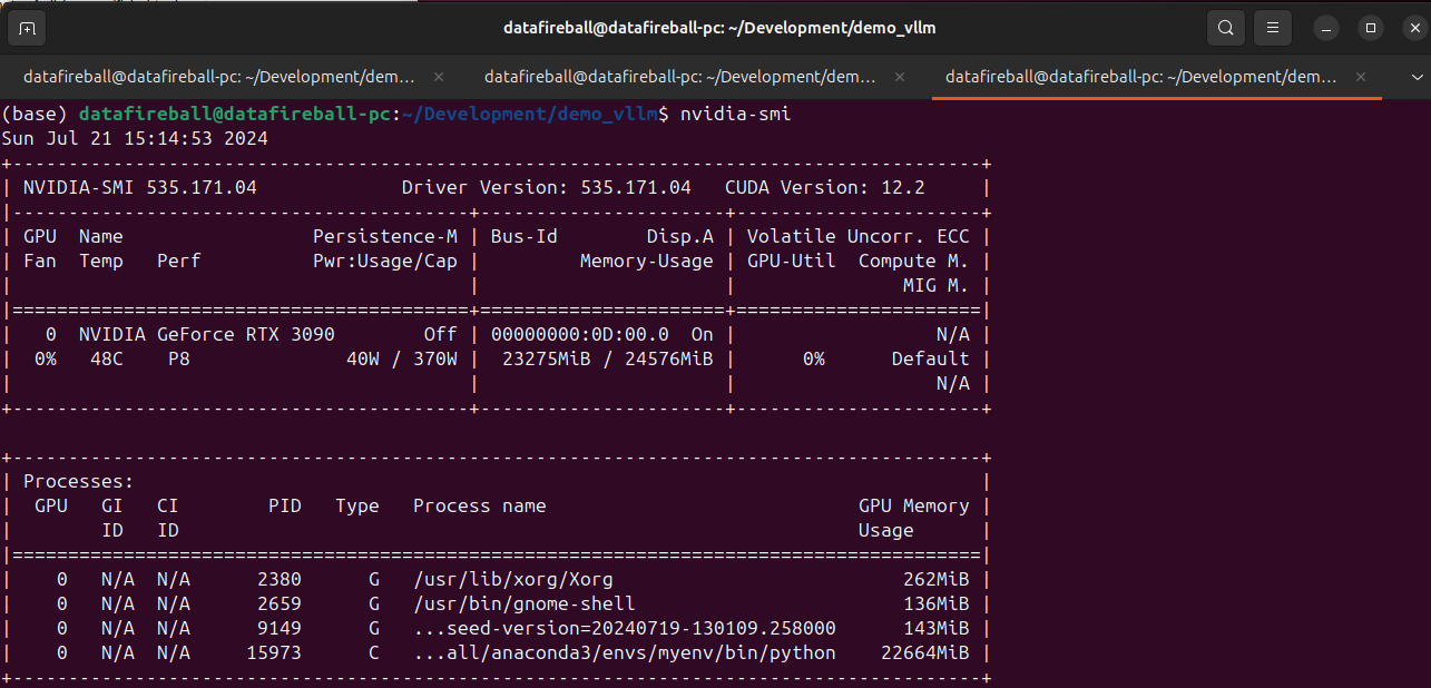
2. Check VRAM and GPU
make sure you have sufficient VRAM to host the model. Here I have a 3090 with 24GB VRAM.
3. Download the model and Serve
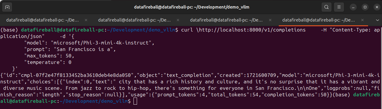
vllm supports many SOTA models, here is a list of all the models that they support. I am testing phi3 microsoft/Phi-3-mini-4k-instruct which is small enough to set up locally. Meanwhile, by downloading the instruct model, I can later refer it within within the gradio chat window to explore the chat experience.
After the model is served, we can interact with the model via API, at this moment, vllm have 3 endpoints implemented, list models (screenshot below), chat completion and create completion endpoints. The vllm API is standardized in a way such that it is a drop in replacement for openai. You can literally take your existing openai code and replace the URL with localhost and your code should just work.
An interesting observation is that the VRAM of 3090 is almost fully occupied, not sure why.
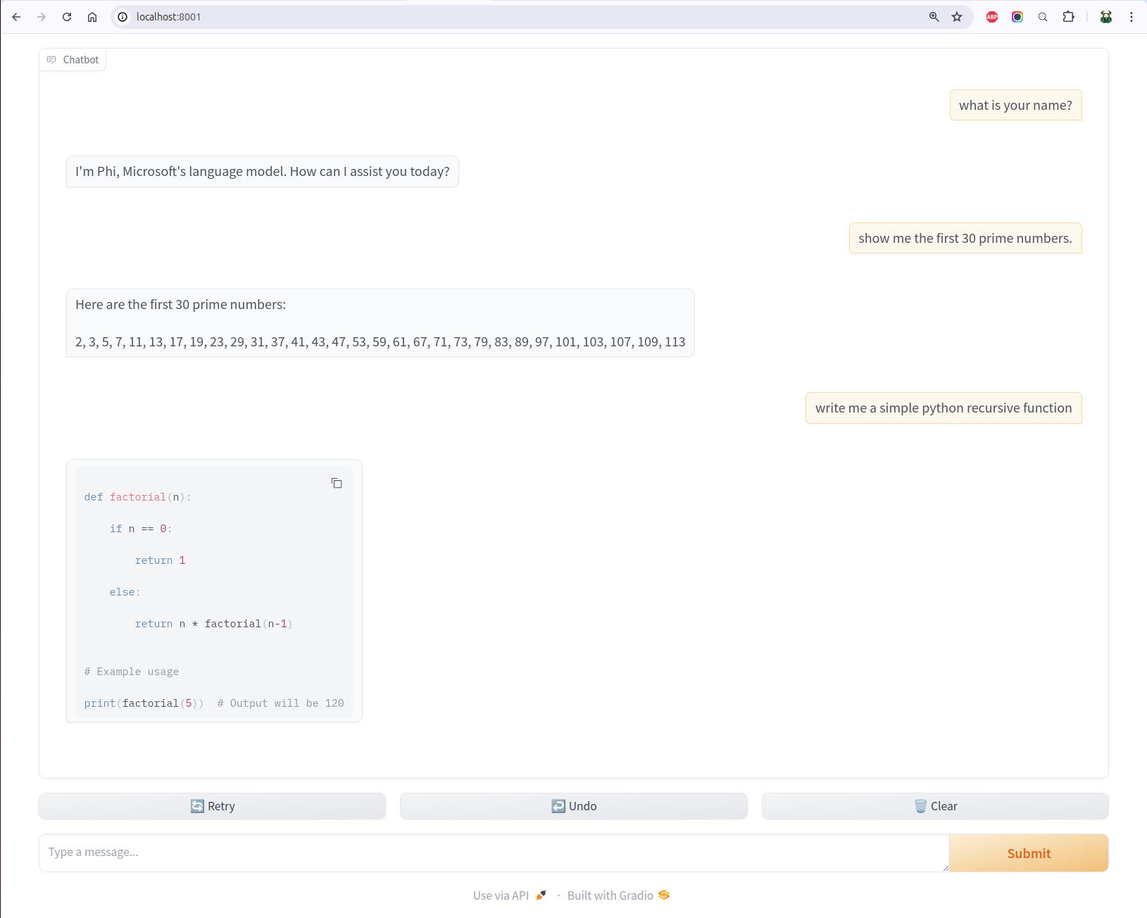
4. Chat UI
vllm comes with many examples. One of the example is to set up a gradio openai chatbot so you can interact with the LLM.
I have heard how even it is to set up model UIs using gradio. By looking into the source code of the UI script, it is so clean and easy, you basically only need to define a predict function by passing it the history and message.
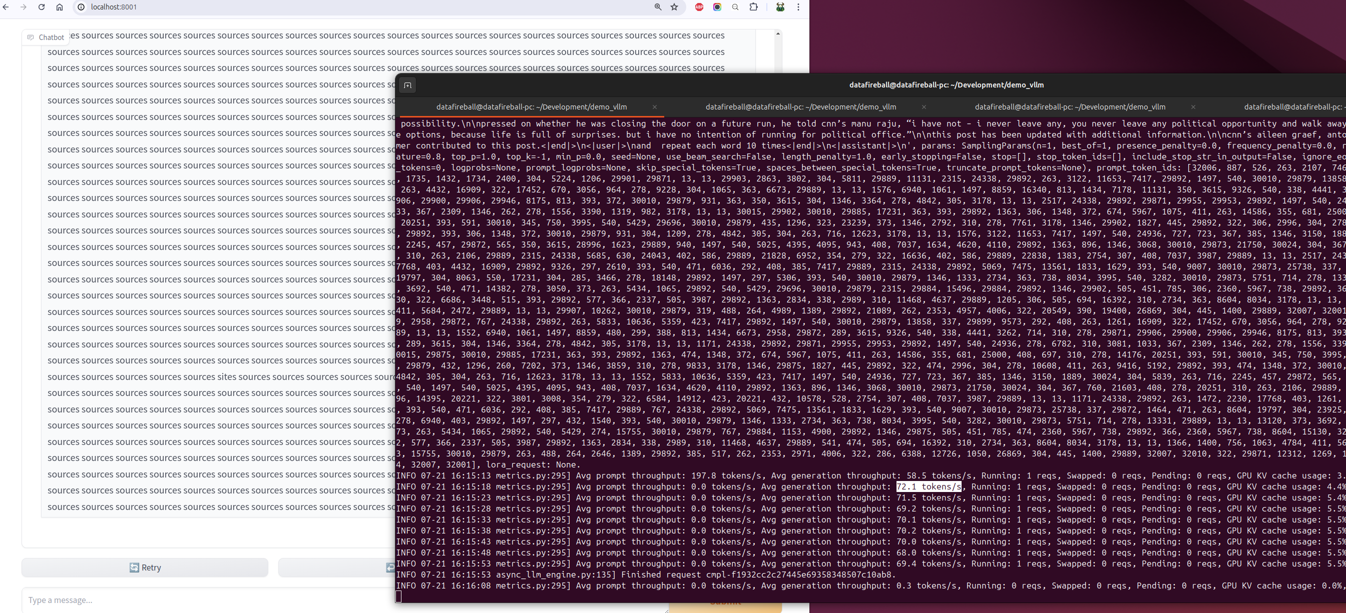
I also tested the throughput by instructing phi to repeat the same word multiple times for a while. During the time of the experimentation, the average generation throughput was about 70 tokens/s.
Just accomplished the short course of pretraining LLM from deeplearning.ai – link
What a good use of a Wednesday night 1 hour’s time, otherwise, I probably will be watching youtube shorts while drinking a beer 🙂
In this tutorial, the instructor Sung(CEO) and Lucy(CSO) from upstage walked through the key steps in training a LLM by using huggingface libraries, mostly importantly, they introduced several techniques like depth upscaling and downsizing to accelerate the pretraining by leveraging weights from existing models but with a different configuration.
The chapter that I personally liked the most is the Model Initialization, this is the step where you customize the configuration and initializes the weights.
For example, here they customized a new model with 16 layers (~308M parameters) and initialized the weights by simply concatenating the first 8 layers from a 12 layers pretrained model and then take the last 8 from the same model. it is like 1,2,3,4, (5,6,7,8,) (5,6,7,8,) 9,10,11,12 and somehow the generate texts have some linguistic coherence instead of completely gibberish.
They claim the depth upscaling and save the training cost by a whopping 70%.
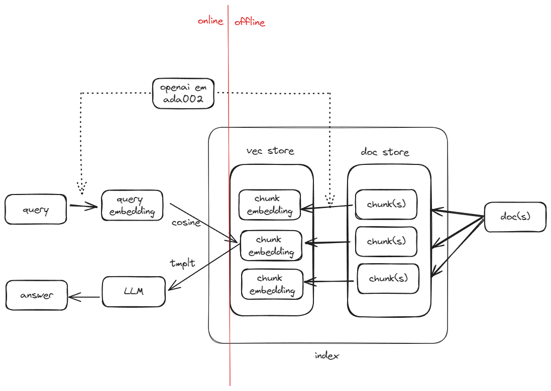
Following the first post of RAG in 5 lines, this post will cover what is happening behind the scene in more detail, what are some of the knobs you can tune so better understand the working internals of llama_index.
llama-index has done such a good job abstracting away the complexities behind the index and query commands. I mentioned that it took me almost 90 seconds to index the 10 articles.
Data Volume
Now let’s look back at how much data that we are working with.
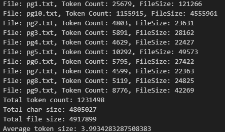
The 10 book occupy about 4.9MB in total in plain text format, by using the cl100k_base BPE, we know they contain in total about 1.2 million tokens. On average, each token takes 4 bytes.
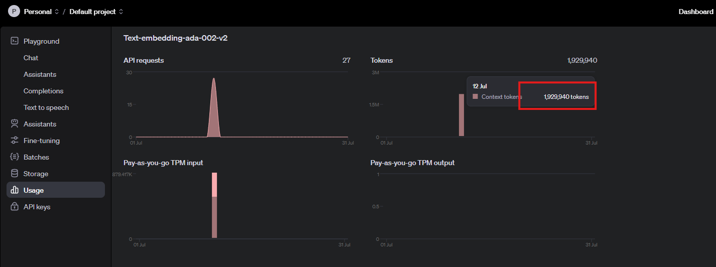
I want to admitthat I had a false start at the beginning. Initially I wanted to index 100 books, then I stopped it after noticing how long the wait was and later changed to 10 books. Now, by noticing that our API usage has 1.9 million tokens in total, that roughly line up with our total number of tokens 1.2 million. (the additional 0.7 million was probably due to my false start).
The theoretical API throughput should be 5M tokens per minute, and our indexing process was about 500K per minute (~10%), this is very slow by default. later on, we can discuss why this happened and how to address it.
Chunk
A key step is RAG is to properly break larger documents into smaller pieces and index them accordingly. In the 5 liner example, there is no place to find the details about how each document is broken down into its own chunks, it is because there are very extensive default settings where the configurations were set there. That means users still have the freedom to customize but if you do not know, there is a default setting for your application.
you can access the default setting by running the following command:
from llama_index.core import Settings
print(Settings)
in the default setting, you can find a lot of useful info like it is using open_ai 3.5turbo as the default LLM and use openai ada002 as the default embedding model. Then you can find they are using the chunk_size of 1024 with a 200 overlap as the sentence splitter.
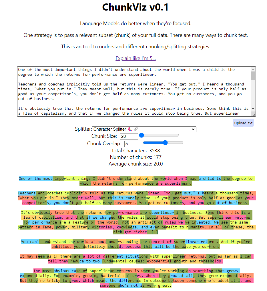
I will not dive too deep into how chunking works, but you should totally check out the ChunkViz from Greg Kamradt.
In the previous section, we know there are about 1.2 million tokens in total. If the chunk size is 1024 with an overlap of 200, we might have ~800 tokens per chunk, which translates to 1.2 million / 800 ~ 1,500 chunks. Now let’s verify whether that was the situation.
>> len(index.docstore.docs)
1583
Document Store
Since now we verified that the raw documents got split into smaller chunks. These smaller documents are now stored in a docstore which is within the index object. as default, the index is using almost a python dictionary which is called SimpleDocumentStore to stores the raw text.
The code below is to iterate through all the docs. Here we print out the first element in the dictionary with its key, its text, number of tokens, and number of characters. Again, we can verify that the token size is within the 1024 chunk size limit and there is on average a 4 to 1 relationship between the number of characters and the number of tokens.
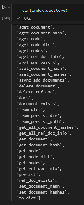
Like any database / store, the document store has many operations mainly around getter/setter, just like the CRUD operations for a database.
Embedding
Embedding is a numerical representation of an entity, in this case, a chunk. based on the default setting, we know they are being batched sent to openai api with a batch size of 100. Given that we have 1,500 chunks, this should translate to 15 requests at most.
Again, it is very likely that we wasted some requests while trying to index 100 docs at the beginning, this verified our hypothesis that the batch indexing is working as expected.
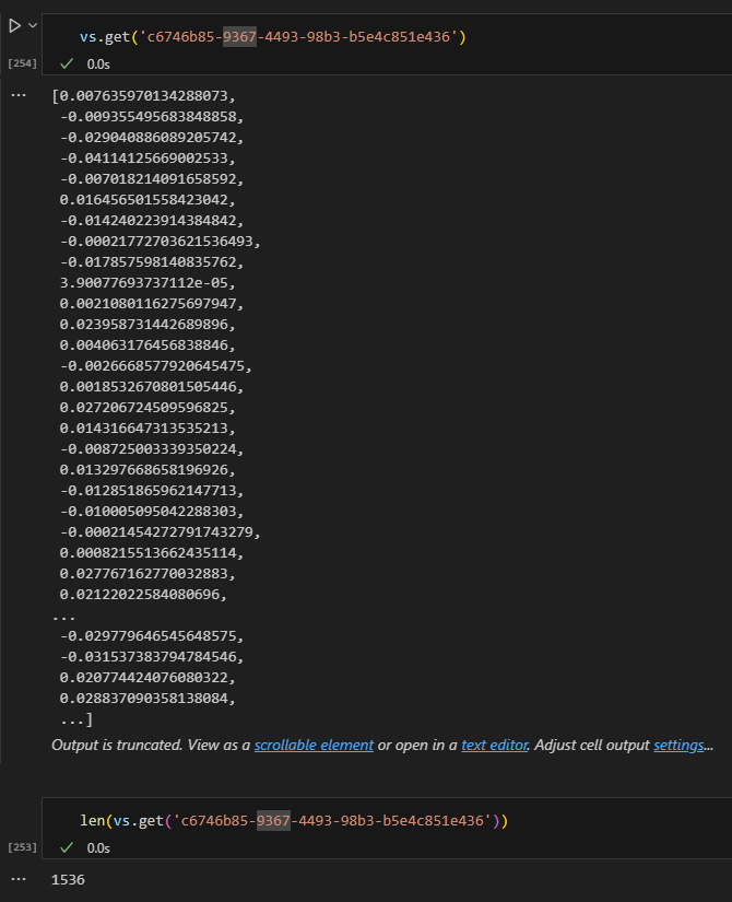
All the embeddings are stored in the vector store.
Vector Store
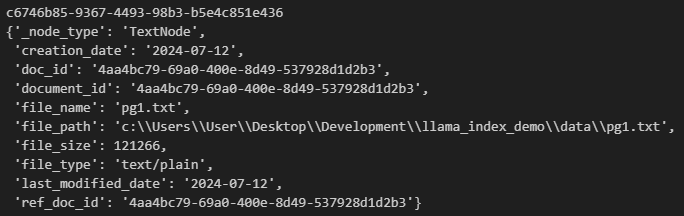
The vector store is yet another place where all the embeddings are stored, in addition, there are a lot of metadata also stored there representing the underlying document.
for k, v in vs.data.metadata_dict.items():
    print(k)
    pprint.pprint(v)
    break
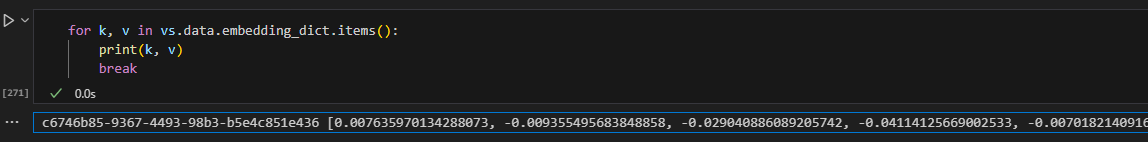
for k, v in vs.data.embedding_dict.items():
    print(k, v)
    break
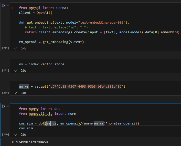
easter egg – not matching embedding
I tried to generate the embedding for a doc myself and compare to its stored embeddings in the vector store, even if they are very similar, I cannot seem to match them 100%. I will not be surprised if there is some pre/post processing somewhere to remove non-printing characters but this is good enough 🙂
Query
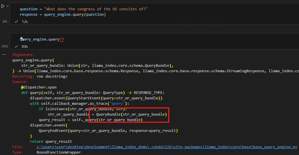
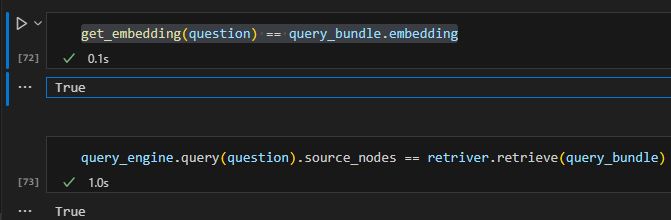
behind the scene of query_engine.query, it converts the query into its embedding and searches it against the vector store to get the best matched record(s). In fact, a simple query_engine will be converted into a retriever which is an synonym in this case.
The code below demonstrated that the query_engine.query will pass in the query as a QueryBundle object.
from llama_index.core.schema import QueryBundle

# Step 1: Generate embeddings for the query
em_query = get_embedding(question)

# Step 2: Create a QueryBundle
query_bundle = QueryBundle(question)

# Step 3: Retrieve nodes using the retriever
retriver = index.as_retriever()
nodes = retriver.retrieve(query_bundle)
Here we directly calculate embeddings for the query using openai api, and then pass the question to initialize a QueryBundle object that will be used to for retrieval.
Now we can have two observations (at least in this simple 5 liner scenario): 1. query_bundle simply takes the query and embeds it 2. the query_engine.query is running retriever.retrieve behind the scene
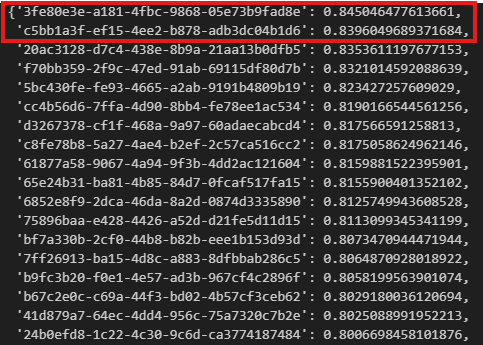
now, let’s try to manually verify the outcome. If we generate the embeddings for the query via openai. Then we can iterate through the vector store and calculate the pairwise cosine similarities, we store the similarities in a dictionary and then we can sort it and highlight the top 2 most similar items.
Based on the outcome, we can verify that the two records 3fe and c5b are the top two results and our similarities match llama-index retrieved too, even their similarity scores match perfectly.
dict_similarity = {}
for k, v in vs.data.embedding_dict.items():
    cos_sim = dot(v, em_query)/(norm(v)*norm(em_query))
    dict_similarity[k] = cos_sim

sorted_dict_similarity = dict(sorted(dict_similarity.items(), key=lambda x: x[1], reverse=True))
sorted_dict_similarity
Synthesis
Now we have located the chunk that is semantically most similar to the query, we still need one more step to further refine in order to provide a concise yet relevant answer. Otherwise, the user is asking “what consistite the US congress”, and we returns a big chunk of text from the constitution for the user to read. This step will need to distill the chunk(s) down to a one or two sentences. In our example, it can even be as short as “house of representative and senate”.
In Llama-index, it is achieved via a component called synthesizer. The retrieved nodes will be served as context, along with the query will be fed directly to a LLM to refine.
l# lama_index.core.prompts.default_prompts.py
DEFAULT_TEXT_QA_PROMPT_TMPL = (
    "Context information is below.\n"
    "---------------------\n"
    "{context_str}\n"
    "---------------------\n"
    "Given the context information and not prior knowledge, "
    "answer the query.\n"
    "Query: {query_str}\n"
    "Answer: "
)
RAG is taking over the world as an augmentation or even replacement to traditional search. It has claims like context augmented leveraging LLM. Through new techniques like LLM and vector search, it offers a new way to offer better quality responses to users. This article is meant to demonstrate how RAG works in the bare minimal example.
Llama-index is one of the the most popular libraries these days for building a rag and its has its famous 5-line starter:
from llama_index.core import VectorStoreIndex, SimpleDirectoryReader

documents = SimpleDirectoryReader("data").load_data()
index = VectorStoreIndex.from_documents(documents)
query_engine = index.as_query_engine()
response = query_engine.query("Some question about the data should go here")
print(response)
Before running the code, we need few preparation steps:
OpenAI Key
To leverage the LLM part, the easiest way is to just call openai api, once you create a key and place it under .env file, you can load into the environment variable as a best practice.
import os
import dotenv
dotenv.load_dotenv()
print(os.environ['OPENAI_API_KEY'])
Books Data
We need some toy data to work with, Gutenberg books is a good place to get some free books. The code below will download the first 10 books from gutenberg project by manipulating the url. The books will be stored in a local directory – data. (precreate it if it does not exist yet)
number_of_books = 10
for i in range(1, number_of_books+1):
    url = f'https://www.gutenberg.org/cache/epub/{i}/pg{i}.txt'
    response = requests.get(url)
    if response.status_code == 200:
        with open(f'./data/pg{i}.txt', 'w') as f:
            f.write(response.text)
    else:
        print(f'Failed to download {url}')
Load the Data and Index
docs = SimpleDirectoryReader('data').load_data()
index = VectorStoreIndex.from_documents(docs)
query_engine = index.as_query_engine()
The three lines above is all you need to load the data, create an index and set the index to be used as query engine. The index initialization took me a while (1minute and 30 seconds) to index the 10 books. So let’s put it into action.
Query
The first few books that we downloaded happen to literatures at the establishment of the US, which also includes the US consistitution, so lets try to ask a question and see how it works.
>> response = query_engine.query("what does the congress of the US consists of?")
>> response

Response(response='The Congress of the United States consists of a Senate and House of Representatives.', source_nodes=
voila, we got the answer that we need!
In the next post, we will dive into each of the building blocks and understand what is happening behind the scene.