Coefficient of determination(决定系数), which is often called R Squared is a commonly used parameter to determine how well data points fit a curve.

set.seed(100)
x <- 1:100
y <- 2 * x + rnorm(length(x), 0, sd <- 10)
summary(m1 <- lm(y ~ x))

plot(y ~ x, type=”o”, main=”y = 2 * x, white noise sd=10″)
abline(m1, col=”red”)

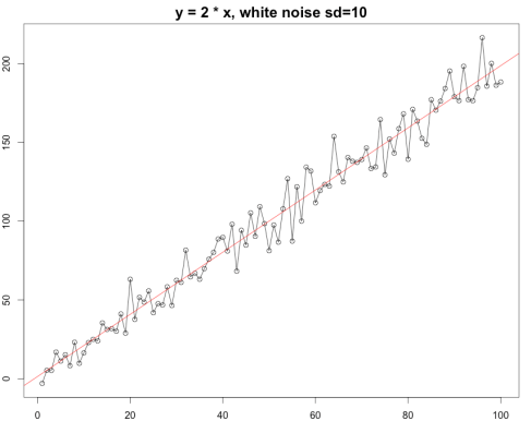
The summary of the linear model m1 looks like below

Call:
lm(formula = y ~ x)

Residuals:
Min 1Q Median 3Q Max
-22.6284 -6.8113 -0.2093 6.1186 26.1505

Coefficients:
Estimate Std. Error t value Pr(>|t|)
(Intercept) 1.37592 2.06135 0.667 0.506
x 1.97333 0.03544 55.684 <2e-16 ***
—
Signif. codes: 0 ‘***’ 0.001 ‘**’ 0.01 ‘*’ 0.05 ‘.’ 0.1 ‘ ’ 1

Residual standard error: 10.23 on 98 degrees of freedom
Multiple R-squared: 0.9694, Adjusted R-squared: 0.9691
F-statistic: 3101 on 1 and 98 DF, p-value: < 2.2e-16

As you can see here R-squared is 0.9694 is very close to 1 which indicates that our linear model fit the data pretty well or vice versa.
you can easily calculate the R-squared yourself by doing this(Wikipedia defination):

> 1 - sum(m1$residuals^2) / sum((y-mean(y))^2)
[1] 0.9693628


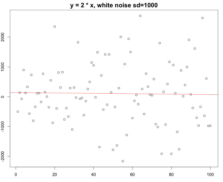
Again, if you change the standard deviation from 10 to 1000, which means that the white noise actually beat the existing rule.. to be simple, there is not that much linear regression during that data range.  You can still build a linear model on it but the R squared turned out to be really really small.

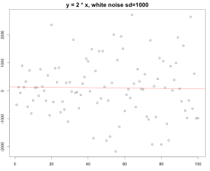
The R squared here is 0.0003613 , which indicates our linear model is really a bad model to fit the datasets.

The model says the slope is -0.6669 which is complete nonsense…

In conlusion, R-squared gives a pretty good idea of how the data points line up with your model.

Then the question is where does the name R – squared come from?

The R is actually Pearson product moment correlation coefficient (Pearson’s R), whose definition is the covariance divide by the product of their own standard deviation.

r <- cov(x, y, method=”pearson”) / (sd(x)*sd(y))

> r^2

[1] 0.9693628

Which lines up perfectly with the R-squared in our linear model above(sd=5).

(References: Pearson Correlation Coefficient, Coefficient of Determination.)