Sympy – Solver

Want to solve a equation using Python, Sympy solver is an easy solution. (I wish twenty years ago I had access to this library so I might do a better job for my school homework)

Screen Shot 2018-01-13 at 6.17.25 AM.png

I am taking a course fundamentals of supply chain from MIT on EDX, there is a small math equation at the beginning of the course when you need to calculate the coefficients for a SKU distribution following power law. To be more specific, the question assumes the distribution follows the power law y = a * x^b where y denotes the percentage of the  items sold and x denotes the number of products sold. At a high level, this is a law behind a few popular products encompass majority of your sales.

Consider the example of a store where 5% of the products account for 66.6% of the items sold, and 50% of the products account for 95% of the items sold. – Course

In this case, we substitute x and y with the real store data, we have

0.666 = a * (0.05)^b
0.95 = a * (0.5)^b

Two variables, two independent equations. You can solve this equation by cancelling any unknown variable. Say let’s get started with cancelling variable a first. We have:

(0.05)^b / 0.666 = (0.5)^b / 0.95

Then we take the natural logarithm of each side, we have:

b * ln(0.05) - ln(0.666) = b * ln(0.5) - ln(0.95)

Finally we got,

b = (ln(0.95) -ln(0.666)) / (ln(0.5) -ln(0.05)) = 0.154

a = 0.95 / (0.5^0.154) = 1.06

Double check, a * (0.05)^b = 1.06 * (0.05)^0.154 = 0.668 ~ 0.666 (pretty close, probably because of the rounding which tends to get amplified in non-linear equations).

Well, as you can see, this equation is not the end of the world but it took me about 10 minutes to write down the equation and punch many buttons on my calculator to get the intermediate steps and what if I just want to get the result.

Here is how you can use Solver to get the result in a faster, more consistent and accurate way:

Screen Shot 2018-01-13 at 6.50.45 AM

Here we go, 5 lines of code, do I really need to explain what happened? I do not think so, right? 🙂

Sympy seems like to have way more functionalities other than just solving elementary school algebraic problems, it also claims to cover ordinary differential equations, partial differential equations, system of polynomial equations and more than that.

(BTW, if you just want to quickly get your hands dirty, Sympy has a live code shell where you can test out the example code or your own problem)


RL Trading – code study of sl-quant

There is this very interesting post from Hackernoon where the author built a self-learning trading bot that will learn and act accordingly to maximize the reward. The post is very fun since demonstrated the learning capability under a few naive models. On the other hand, it is actually the underlying implementation that intrigued me the most which I decided write this blog and go through the notebook provided by Daniel and learn more what is happening under the hood.

Reward

Screen Shot 2018-01-08 at 10.33.37 PM

The get_reward function is probably one of the most important steps in designing a reinforcement learning system. In an trading example, it can be somehow straightforward at first glance because people can simply use the financial position ( like P&L) as the measurement, actually it is probably the one method many people will agree and adopt.

We can start by first looking into the terminal_state == 1 part of the code, which indicates that is the last step of the process. In this case, the author simply call the Backtest function straight out of box by passing in pricing information and the signal information, in this case, each element of xdata stores the state which contains the current price and the difference comparing with the previous day. Hence, [x[0] for x in xdata] is a list of all the prices. In this case, you can grab the P&L data for the last day and you are good to good. (click here to learn more about the backtest functionality within twp)

The most interesting part is actually by looking into how the intermediate steps rewards are calculated. Within the terminal_state = 0, there are two if statements all based on the value of signal[timestep] and signal[timestep-1]. Signal is “Series with capital to invest (long+,short-) or number of shares”. In that case, signal[‘timestep’] and signal[timestep-1] is the capital to invest for the current and previous step. The interesting part if the both of them are equal to 0, basically means nothing to invest, the author actually deduct 10 points from the reward variable, I think this is to penalize the activity of doing nothing probably. Then, the step of where the signal for today and yesterday are different, this is probably the most challenging part of this reward function.

It built a while loop and go backwards in time to compare the two consecutive days of signal until they are equal. Actually, if the previous step and the one before it happen to have no change. Then i = 1 and it jumped out of the loop and stays at 1. However, if this is a very active investor and every day is different. i could increase to be as large as timestep – 1.  The code screenshot got cut off and here is the complete code for line 94.

Screen Shot 2018-01-08 at 11.01.48 PM

Here I am having a hard time understanding how this reward function is established. I can understand the price difference part. And multiply by the number of shares gives you basically the profit, or loss if there is a price drop. At the beginning, I thought the author must really hate making money because he multiplied that profit by a negative 100. Later on, I realized that the signal is interesting, it could be a positive number which means the investor is in a long position of owning certain stocks and a negative number indicates the investor is in a short position cashing out his stocks. So if this person is selling, then signal is negative, and if the price increased, this actually ended up a big positive boost to the reward. +price * -share * – 100 = +100 P&L. Last but not least, he also added a component where he multiply the number of shares he owns yesterday by the number of days that he hold and divide by 10. This is also a positive number and grows linear as the number of days he holds this position (i) and by the absolute value of his position. Bigger the deal is, and this will lead to a bigger reward. In this way, how this second component in the reward function is structured probably will boost the performance of holding a big amount of stocks for a long time. This is interesting because the reward function is crafted in such a way that encompass several key data points but in the end, it will collapse back to the P&L, I am wondering why he did not use P&L just across the who journey.

All things said, this is actually one way of how reward function got implemented.

evaluate_Q

Screen Shot 2018-01-08 at 11.29.39 PM

So here, the inputs to the evaluate_Q function are a trained prediction model – eval_model and a eval_data, which is a list containing a time series of pricing information.

First, the variable got initialized into an empty panda series. and then the pricing info got to be used to initiate the xdata (a time series of all the states) in which variable state got initialized to be the first state. Next comes the grand while loop that will not terminate until the end. Each loop represents a time step, a day, a minute, or a second given how your time step is defined. At the beginning of the loop, the model will be used to predict the Q value for the given state. This will generate a value for each action taken under that state. In this case, we have only 3 different actions, buy, sell or hold. In this case, the eval_model.predict is supposed to generate a score Q value for each of those action taken. Whichever has the highest score will be deemed as the best action and be acted upon. Given the action taken, this will bring the process into the next state – new_state, time_step will increase by one and the signal variable will also be updated within the take_action function. In this case, the signal variable keep appending and appending until the end of the simulation. The eval_reward is actually calculated at every step and actually only eval_reward in the last loop got used.  In my point of view, maybe the author should move that part of the code outside the while loop to improve some efficiency.

Main

Screen Shot 2018-01-08 at 11.50.40 PM

This is where the magic happens. First, it is the signal got initialized to be an empty panda series. Then it goes into a for loop, and the number of the loops is depending on how many epochs the user wants this model to run. Within each epoch, all the key variables got reinitiated but seems like signal variable got to escape from this process.

Within each epoch, there is this while loop looping through each state. This part of the code is actually fairly similar to evaluate_Q, you will see as we read more. First the model is being used to predict the Q value, however, before the Q value got used to pick the next optimized action. There is a random factor for exploration where there is chance that the next action will be randomly chosen to avoid local optimal or overfitting. Otherwise, actually most of the cases assuming you picked up a fairly small epsilon, the next action will be based on the estimation of the Q value. After the action being taken, all the key variables should be updated and we will land in a new state, then the new state will be used to predict the next Q value and now we can calculate the update to be the reward for the current step plus the best estimation for the next step at that time. Then this cycle will be fed to the prediction model and further enhance its capability to predicting the Q value for a given state and the right action to take.

Screen Shot 2018-01-09 at 12.06.21 AM

Again, I just want to highlight that how the recursion happened here. Probably a whole article should be contributed here to explain the mathematical reason behind how the model is updated and why the update is the reward with an attenuated future Q value. If you want something quickly and dirty, this stackoverflow is help explaining the difference between value iteration and policy iteration from the implementation perspective.

This is basically it, a more detailed explanation of the source code behind the interesting post about self learning quant.

Reference:

twp – Backtest module Part 1

twp – tradeWithPython is a utility library meant to help quant who uses Python. You can find the source code here and the documentation here. This library has been used by several projects so I am going to take a dive into the backtest module and show how to use it (given the author did not put too much thought into the documentation, or he thought it is already straightforward enough :)) .

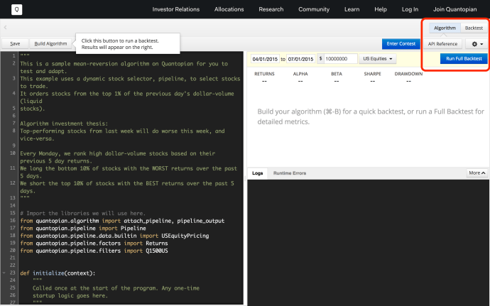
You can find the source code for the backtest module here. At a high level, backtesting in the financial realm refers to “estimate the performance of a strategy or model if it had been employed during a past period.” This will enable quants to quickly evaluate any given investing strategy without conducting real experiment nor waiting for another significant amount of time while still gain some real life insight with confidence by doing simulation on existing data. For example, backtest is the first class citizen of the popular algo platform quantopian.

quantopian_backtest

Anyway, now you understand how important backtest is in testing algo now, let’s go through the source code twp.backtest to look through how a backtest module got implemented and what are the key metrics got captured there.

Let’s take a look at the class Backtest directly, the constructor itself has included all the key data elements outright.

Screen Shot 2018-01-07 at 4.38.12 PM

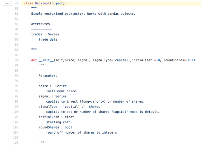
Price is a panda Series which contains the time series of pricing information. If we are looking at stock price, pd.Series([1,2,3,4,5]) could represent the information that the given ticker is $1 per share on the first day, say Monday, has a one dollar increment for the rest of the week, ended $5 dollar on Friday. Signal is a variable that contains the financial activity or trading operation, for example, [NA, NA, 3, NA, -2] is a valid Signal variable which can be interpreted as the investor is in a long position of three shares of stock on the third day and in a short position of two shares on the last day, assuming the signal type is “shares” versus “capital”. The rest of the parameters are fairly easy to understand.

Now lets look at the body of the source code of the constructor:

Screen Shot 2018-01-07 at 4.46.34 PM

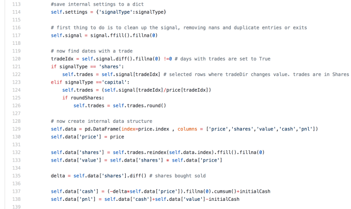
At line 117, signal got “cleaned up” by call ffill() followed by fillna(0). These two methods used in conjunction is very common for dealing with time series information with missing values. Using the example where signal = [NA, NA, 3, NA, -2] again, ffill() is the same as locf in R, which in essence is to fill the missing value with the last non missing value. However, for the leading missing values, like the first two NAs in our example, there is no preceding valid value, then it will stay NA. After that, fillna will replace all the NAs, in this case, the leading NAs with whatever value got passed along, which is set to 0.

Screen Shot 2018-01-07 at 4.54.53 PM

Next is the tradeIdx variable, it is basically the difference between every two pair of consecutive elements so theoretically, tradeIdx is exactly one element shorter than signal. However, for the very first element of the Series, there is no element prior to it to subtract with, it will be filled with NA so it has the same length as the input Series. Then fillna(0) will replace NA with 0 right after that.

Screen Shot 2018-01-07 at 5.15.55 PM

Then tradeIdx will be used to slice the signal and store the trade into the variable self.trades, keeping the index number.

Now, let’s talk about the “shares” variable. It was calculated in this way

tradeIdx = signal.ffill.fillna.diff.fillna != 0
trades = signal[tradeIdx]
shares = trades.reindex.ffill.fillna

In essence, “shares” is basically “trades” and basically “signal”. So that in case, to calculate the delta, or in another way, on what day did the investor sold the stocks, we need to calculate the difference of shares to calculate the delta.

Screen Shot 2018-01-07 at 5.53.33 PM

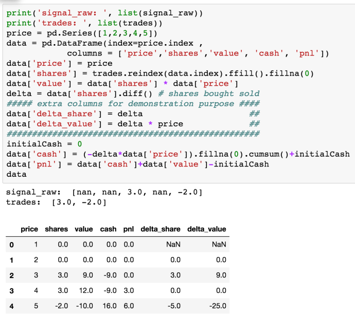
The screenshot above clearly explained how it looks like. And let’s translate the verbose code into plain English, which might be a bit easy to interpret. In the end, this basically describe a  scenario where this person netted $6 by borrowing money to buy 3 shares of stock on the third day. And flipped it on the last day, where the price per share increased by 2 dollar. That left a $6 net profit on the book. At the same time, this person not only sold all the shares he borrowed, he is even in a position of “-2” on the last day, which indicates that he sold some shares that he even does not own. He could be borrowing two shares from somebody else at the value price of $5. He could have sold it on the next day and then buy it back in a future when the price is low, in that case, this person can not only pay back the two shares to its original owner but also profit since the he is in a short position and the price dropped in his favor.

Let’s give another example with some initial cash say $100 at the beginning and put this person in a short position given a growing underlying stock price – unlucky.

Screen Shot 2018-01-07 at 6.03.43 PM

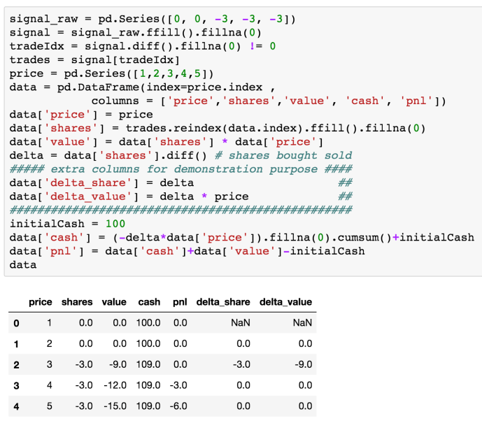
As you can see, this person borrowed and cashed out some stock on the third day, -9 on value and 109 on cash. Then the underlying price of stock keep going up and the three shared that he owned used to worth 9 dollars now he is in the situation which he owes 15 dollar worth of stock, which net a loss of 6 dollars.

Sharpe

Screen Shot 2018-01-07 at 6.16.28 PMScreen Shot 2018-01-07 at 6.16.47 PM

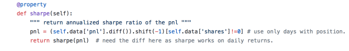
Then in the backtest, the author implemented a method for a class called sharpe and there is also a utility function defined outside the class called sharpe with an argument which is the daily sharpe ratio, it basically convert from daily to annualized sharpe.

Screen Shot 2018-01-07 at 6.28.59 PM

Today, we have covered the majority of the logical part of the backtest module, however, there are still a few functions like plotting that we need to further evaluate in the second part of the tutorial.