R – Dplyr tutorial from Data School

Here is a fantastic video tutorial of Hadley Wickham’s dplyr package from Data School.

R – Lattice, Trellis another awesome framework for data visualization.

This whole post originates from this stackoverflow question. The original poster(OP) was having a hard time putting multiple `plots` into the same canvas. It looks like he was using the base plot function and I assumed the par(mfrow) will be enough in that case. However, it turned out this is a way more interesting question than I first realized and here are all the `aha`s.

He was using a library called DoseFinding , which is

a package provides functions for the design and analysis of does-finding experiments(for example, pharmaceutical Phase II clinical trials).

In there you can use the base plot function to plot the return object from the function `fitMod` (the does response model). You can see the return class of fitMod is called “DRMod” (drug response model) and the plot class is called “Trellis”.

Actually, Trellis is a whole visualization framework developed by the Bell Lab and AT&T Research. Here is another post to understand post to give you a basic understanding of lattice and trellis.

I have working working with the base plot functions like boxplot, hist, plot.. and also ggplot2 from Hadley Wickham for a while, and I am surprised to find out how easy it is to use lattice package to draw plots taking multiple variables into consideration.

bwplot( mpg ~ cyl.f | gear.f * am)

ggplot(data=mtcars, aes(x=as.factor(cyl), y=mpg)) + geom_boxplot() + facet_wrap(~gear + am)

There are also so many different plot methods in lattice, which you can spend more time exploring.

R – Shinyapps.io A free Platform to host your ShinyApp

shinyapps.io is another product (alpha version now) from RStudio, where it will host shiny apps for you free. You just need to install the package shinyapps, login, and you can just run command `deployApp()`. Then you will have your app running 24 * 7.

shinyappsio dashbaord

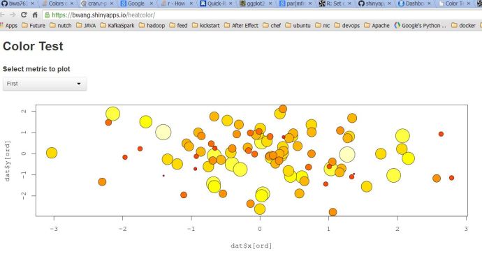
a shinyapps.io hosted shinyapp Code borrowed from Stackoverflow

The Shiny application code was borrowed from this stackoverflow question.

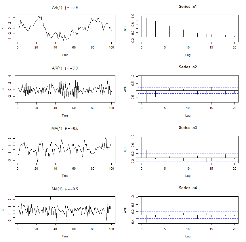
STATS – How a Auto Regressive Series and Moving Average Series Look Like

ACF of AR(1) is phi^h

ACF of MV(1) is theta/(1+theta^2) only for h=1 and 0 when h>1

——————————————————————————————–

par(mfrow=c(4,2))
a1 <- arima.sim(list(order=c(1,0,0), ar=0.9), n=100)
plot(a1, ylab=”x”, main=(expression(AR(1)~~~phi==+.9)))
acf(a1)
a2 <- arima.sim(list(order=c(1,0,0), ar=-0.9), n=100)
plot(a2, ylab=”x”, main=(expression(AR(1)~~~phi==-.9)))
acf(a2)
a3 <- arima.sim(list(order=c(0,0,1), ma=0.5), n=100)
plot(a3, ylab=”x”, main=(expression(MA(1)~~~theta==+.5)))
acf(a3)
a4 <- arima.sim(list(order=c(0,0,1), ma=-0.5), n=100)
plot(a4, ylab=”x”, main=(expression(MA(1)~~~phi==-.5)))
acf(a4)

Stats – What is “R squared” and what is the “R” in “R squared”

Coefficient of determination(决定系数), which is often called R Squared is a commonly used parameter to determine how well data points fit a curve.

set.seed(100)
x <- 1:100
y <- 2 * x + rnorm(length(x), 0, sd <- 10)
summary(m1 <- lm(y ~ x))

plot(y ~ x, type=”o”, main=”y = 2 * x, white noise sd=10″)
abline(m1, col=”red”)

The summary of the linear model m1 looks like below
Call: lm(formula = y ~ x)

Residuals:
Min 1Q Median 3Q Max
-22.6284 -6.8113 -0.2093 6.1186 26.1505

Coefficients:
Estimate Std. Error t value Pr(>|t|)
(Intercept) 1.37592 2.06135 0.667 0.506
x 1.97333 0.03544 55.684 <2e-16 ***
—
Signif. codes: 0 ‘***’ 0.001 ‘**’ 0.01 ‘*’ 0.05 ‘.’ 0.1 ‘ ’ 1

Residual standard error: 10.23 on 98 degrees of freedom
Multiple R-squared: 0.9694, Adjusted R-squared: 0.9691
F-statistic: 3101 on 1 and 98 DF, p-value: < 2.2e-16

As you can see here R-squared is 0.9694 is very close to 1 which indicates that our linear model fit the data pretty well or vice versa.
you can easily calculate the R-squared yourself by doing this(Wikipedia defination):
> 1 - sum(m1$residuals^2) / sum((y-mean(y))^2) [1] 0.9693628

Again, if you change the standard deviation from 10 to 1000, which means that the white noise actually beat the existing rule.. to be simple, there is not that much linear regression during that data range. You can still build a linear model on it but the R squared turned out to be really really small.

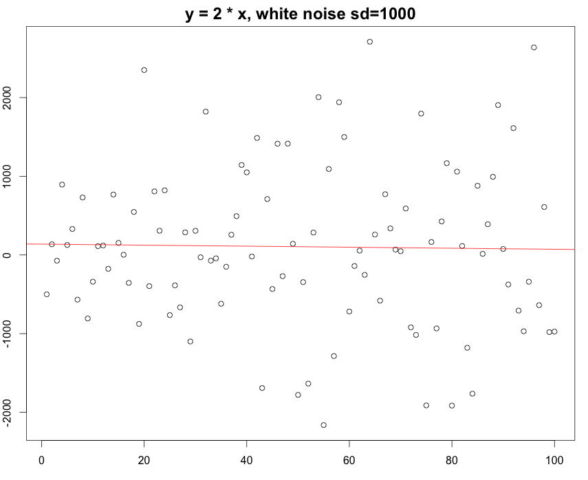
The R squared here is 0.0003613 , which indicates our linear model is really a bad model to fit the datasets.

The model says the slope is -0.6669 which is complete nonsense…

In conlusion, R-squared gives a pretty good idea of how the data points line up with your model.

Then the question is where does the name R – squared come from?

The R is actually Pearson product moment correlation coefficient (Pearson’s R), whose definition is the covariance divide by the product of their own standard deviation.

r <- cov(x, y, method=”pearson”) / (sd(x)*sd(y))

> r^2

[1] 0.9693628

Which lines up perfectly with the R-squared in our linear model above(sd=5).

(References: Pearson Correlation Coefficient, Coefficient of Determination.)