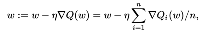
The regularization is a trick where you try to avoid “overcomplexing” your model, especially during the cases in which the weights are extraordinary big. Having certain weights at certain size might minimize the overall function, however, that unique sets of weights might lead to “overfitting” where the model does not really perform well when new data come in. In that case, people came up with several ways to control the overall size of the weights by appending a term to the existing cost function called regularization. It could be a pure sum of the absolute value of all the weights or it could be a sum of the square (norm) of all the weights. Here is usually a constant you assign to regularization in the cost function, the bigger the number is, the more you want to regulate the overall size of all the weights. vice versa, if the constant is really small, say 10^(-100), it is almost close to zero, which is equivalent of not having regularization. Regularization usually helps prevent overfitting, generalize the model and even increase the accuracy of your model. What will be a good regularization constant is what we are going to look into today.

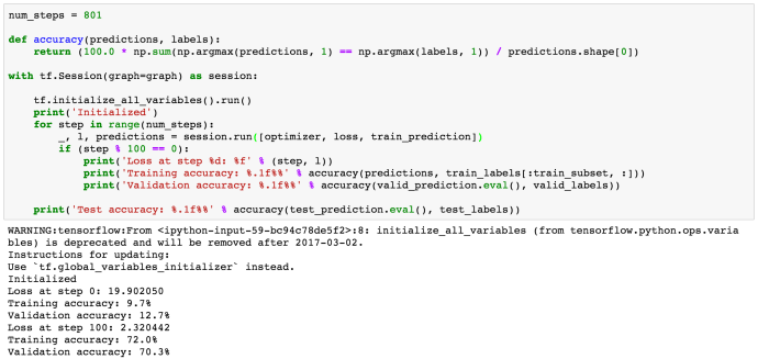
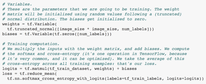
Here is the source code of regularizing the logistic regression model:

logits = tf.matmul(tf_train_dataset, weights) + biases
loss_base = tf.nn.softmax_cross_entropy_with_logits(labels=tf_train_labels, logits=logits)
regularizer = tf.nn.l2_loss(weights)
loss = tf.reduce_mean(loss_base + beta * regularizer)
optimizer = tf.train.GradientDescentOptimizer(0.5).minimize(loss)

As you can see, the code is pretty much the same as the one without regularization, except we add a component of “beta * tf.nn.l2_loss(weights)”. To better understand how the regularization piece contribute to the overall accurarcy, I packaged the training into one function for each reusability. And then, I change the value from extremely small to fairly big and recorded the test accuracy, the training accuracy and validation accuracy on the last batch as a reference, and plotted them in different colors for each visualization.

The red line is what we truly want to focus on, which is the accuracy of the model running against test data. As we increase the value from tiny (10^-5). There is a noticeable but not outstanding bump in the test accuracy, and reaches its highest test accuracy during the range of 0.001 to 0.01. After 0.1, the test accuracy decrease significantly as we increase beta. At certain stage, the accuracy is almost 10% after beta=1. We have seen before that our overall loss is not a big number < 10. And even the train and valid accuracy drop to low point when the beta is relatively big. In summary, we can make the statement that regularization can avoid overfitting, contribute positively to your accuracy after fine tuning and potentially ruin your model if you are not careful.

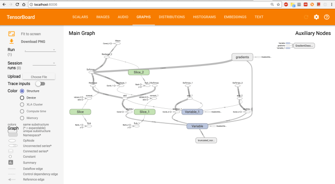
Now, let’s take a look at the how adding regularization performed on a neural network with one hidden layer.

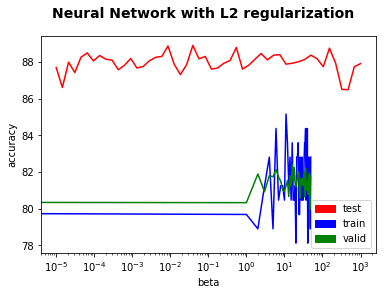
First, we want to highlight that this graph is in a different scale (y axis from 78 to 88) from the one above (0 to 80). We can see that the test accuracy fluctuate quite a bit in a small range between 86% to 89% but we cannot necessarily see a strong correlation between beta and test accuracy. One explanation could be that our model is already good enough and hard to see any substantial change. Our neuralnet with one hidden layer of a thousand nodes using relu is already sophisticated, without regularization, it can already reach an accuracy of 87% easily.

After all, regularization is something we should all know what it does, and when and where to apply it.

The homework of fullyconnected session require the students to:

Turn the logistic regression example with SGD into a 1-hidden layer neural network with rectified linear units nn.relu() and 1024 hidden nodes. This model should improve your validation / test accuracy.

The last block of code was neural network where is simply a network connecting input directly to the output, of course, softmax in the middle. And the change we need to make here is to instead of mapping all the inputs (784) to (10) outputs, we first need to create a layer which maps 784 to 1024 and then another layer to map 1024 to 10. Nothing fancy, but we simply need to add relu after the first Wx+b before passing on to the next layer as the activation function.

First, let’s take a look at how the old no hidden layer SGD looks like:

# Variables.
weights = tf.Variable(
    tf.truncated_normal([image_size * image_size, num_labels])
)
biases = tf.Variable(
    tf.zeros([num_labels])
)

# Training computation.
logits = tf.matmul(tf_train_dataset, weights) + biases
loss = tf.reduce_mean(
    tf.nn.softmax_cross_entropy_with_logits(
        labels=tf_train_labels, 
        logits=logits
    )
)

# Optimizer.
optimizer = tf.train.GradientDescentOptimizer(0.5).minimize(loss)

# Predictions for the training, validation, and test data.
train_prediction = tf.nn.softmax(logits)
valid_prediction = tf.nn.softmax(tf.matmul(tf_valid_dataset, weights) + biases)
test_prediction = tf.nn.softmax(tf.matmul(tf_test_dataset, weights) + biases)

Now, let’s build on top of this and see if we can architect a new network based on the homework requirement. Frankly speaking, the answer I am going to provide here was mostly inspired by this notebook or even more, the answer is only a fraction of what Mr. Damien offered in his code.

First of all, our network was like softmax(w * x + b) before. Now we are going to have one extra layer. The math will look like softmax(w_2 * h+b_2) where h = relu(w_1 * x + b_1). Or put everything in one:

softmax(w_2 * relu(w_1 * x + b_1) + b_2)

It is a bit complex, but not too much. we first need to redefine the variable weights and bias in a way where all of the four variables w_1, w_2, b_1, b_2 are included.

w_1 now is of the dimension (784, 1028) and b_1 has the size of (1, 1028)
w_2 is of dimension (1028, 10) and b_2 is of size (1, 10). Keep the right dimension in mind, we need to create four variables where two of the weights need to be initialized by normal distribution where the biases can be initialized by zeros, just like the old days.

After that, here comes to developer’s personal preference. You can put all the variables into a dictionary say “myvariables” where it stores all the weights and biases. Or you can create two variables “weights”  and store the two weight variables within that weights dictionary. And the same for biases. Or create one variable all separately and pass them around whenever you need them. First of all, all the design preferences will work in the end if you implement them properly. Damien’s code was following the second design type, which looks clean and tide. Here I am going to package all the variables in one dictionary just to be different.

# Variables
myvars = {
 'w_h': tf.Variable(tf.random_normal([n_input, n_hidden])),
 'b_h': tf.Variable(tf.random_normal([n_hidden])),
 'w_o': tf.Variable(tf.random_normal([n_hidden, num_labels])),
 'b_o': tf.Variable(tf.random_normal([num_labels]))
}

Now we are done initializing our variables, the next step is to build the model, or how we are going to predict using all the variables that we just defined. In the network without hidden layers, it was easy and actually a one liner

logits = tf.matmul(tf_train_dataset, weights) + biases

In our case, it will look like this:

layer_hidden = tf.add(
    tf.matmul(x, myvars['w_h']), 
    myvars['b_h']
)
logits = tf.matmul(
    tf.nn.relu(layer_hidden), 
    myvars['w_o']
) + myvars['b_o']

Theoretically you can put everything into one liner to make the statement that “it is still a one liner”, but I highly suggest we at least break them down into components that are more readable. In this case, breaking them down into layers is probably a good idea.

Actually, this block of code will be reused quite a few times other than defining the logits, you will use the model when building accuracy, testing against validation, test, ..etc. So let’s build them into a function:

def model(x, myvars):
    layer_hidden = tf.add(tf.matmul(x, myvars['w_h']), myvars['b_h'])
    logits = tf.matmul(tf.nn.relu(layer_hidden), myvars['w_o']) + myvars['b_o']
    return logits

The definition of loss function and even optimizer is totally independent of how the neural internally looks like internally:

pred = multilayer_perceptron(tf_train_dataset, myvars)
loss = tf.reduce_mean(
    tf.nn.softmax_cross_entropy_with_logits(
        logits=pred, 
        labels=tf_train_labels
    )
)
optimizer = tf.train.GradientDescentOptimizer(0.5).minimize(loss)

After all, we need to define the accuracy against training, validation and testing. Since we have packaged our model into one function, our implementation for a network even with one hidden layer is even cleaned than the homework itself. This is how it looks like right now:

train_prediction = tf.nn.softmax(pred)
valid_prediction = tf.nn.softmax(model(valid_dataset, myvars))
test_prediction  = tf.nn.softmax(model(test_dataset,myvars))

Now we have our new model. And the way we structured our code now, you only need to modify model function and add more variables to myvars even want to add more layers. Everything else should stay exactly the same. When we run our code, the accuracy got improved quite a bit, by about 10% (from 80% to 90%). And the performance difference between GPU and CPU is really substantial. Attached are two screenshots to demonstrate the performance difference between GPU (4 secs) and CPU (37 seconds).

This slideshow requires JavaScript.

After playing with tensorflow example codes quite a bit, I think I am ready, and actually cannot wait to unleash the power of GPU. There are so many benchmarks here and there where people brag about how GPU kicks CPU’s ass when it comes to massive computation tasks. I threw a few hundred bucks into my first GPU purely to play top notch video games – Starcraft II back when it first came out, thanks to Blizzard entertainment. Using GPU for machine learning is purely a afterthought, looking back.

This weekend, I brought a GPU workstation back home. However, after being put off by my wife telling me that “I do not want you to make mess in our living room, you can not put anything on the table….”. The sad part, the workstation does not have wireless internet connection, and what is even worse, we only have ethernet connection right next to the router in the living room. Take all constraints into consideration, the only option left here is to leave the desktop as a remote server and access it through other devices (other computers within the same network).

Thank goodness, it was quite easy to set up any Ubuntu machine to be accessed through ssh. Actually, there is no need to set up remote desktop, since we can use the terminal for anything graphic related like web surfing. The only thing we need to do is set up the desktop as a server, people can ssh in, and for the Python related developer, we also need to set up the desktop as a jupyter notebook server where we are going to conduct our experiment.

As you can see in the end, we merely need to plug a power and ethernet cable to the desktop. The moment you power it on, you should be able to access the desktop via SSH and you can even power it off remotely by issuing comment “sudo shutdown”. Now you can work in your bed and never even come off your bed to shut it down!

Also, to make it slightly easier for consistency access, I suggest you log into the router to reserve an IP so that the desktop will not be assigned to a different IP every time it is reboot or what, due to the fact that DHCP is the default many default devices.

After that, you can SSH into your computer, conda install or pip install to set up the tensorflow CUDA development environment. However, it might still be a PITA to develop without any IDE, and in this case, I will be using jupyter notebook. Jupyter notebook does not handle multi-tenancy that well, say you have multiple people accessing the server at the same time. Jupyterhub is supposed to be the tool to ease that pain and the installation and set up are fairly easy. Since I will the only user within the network, I literally did nothing but ran the command “jupyterhub” and now we have a jupyter notebook running that you can simply enter the address “10.0.0.54:8000” on any laptop within the network (wifi, ethernet,..). And here is how it looks like on my MacBook Pro accessing that GPU desktop:

This slideshow requires JavaScript.

For those curious mind, look at the slideshow above proving that I am running the Udacity fullyconnected notebook and it is actually running on top of a lovely GPU!

The source code is from here. Since the source code was coded to demonstrate the fundamentals of tensorflow which is not necessarily to run the code on GPU. There will not be any proof right out of box any step is actually using GPU (if available GPU and CPU coexist, tensorflow actually will prioritize GPU).

Here is a snippet of code where I want to highlight. tf.ConfigProto, device_count to be 0 will force the machine to use CPU which you can compare with when you have an time consuming task (the notebook was quite fast using either CPU or GPU).

config = tf.ConfigProto(
    log_device_placement=True, 
    device_count = {'GPU': 0}
)
graph = tf.Graph()
with graph.as_default():
 ...
with tf.Session(graph=graph, config=config) as session:
    tf.global_variables_initializer().run()
    ...
    _, l, predictions = session.run([optimizer, loss, train_prediction], feed_dict=feed_dict)
    ...

Also, log_device_placement set to be true will enable detailed logging about operations.

I think this is the end of this post. Nothing new, nothing ground breaking, but quite a fun to see everything got put together, right?

Following the previous posts, this one will be dedicated to go through the block of code which implemented the gradient descent.

First, I want to share my intuitive understanding of how gradient descent works using an analogy. Think about the goal of the optimizer is to find a set of parameters (w, b) in order to minimize the loss function across all the training data. An oversimplified analogy could be trying to find a position within your city that has the lowest altitude. In this case, the altitude is the loss function and the position is the (w,b) which you can control and tweak. The computation for the loss function could be very time consuming across all the training data (think about I want to locate the exact altitude for any given point to the precision of centermeter, or even nanometer). This is precise and accurate of course, but unnecessarily time consuming. After a whole day, you might only be able to measure the altitude of your home to that level of accuracy. The idea of stochastic gradient descent is to trade off the precision for much better speed gain. It is under the assumption that even using a subset of the data, it should still be representative of the general trend of where the loss function is leaning towards and should provide you with a measurement that is in the ballpark. Or in our analogy, I can easily tell you the rough altitude for any given point to the precision of inches or even feet, or meters, at no time. In that case, you do not need to struggle picking the hairs but can quickly realize, your whole neighborhood is not in the lowest point, and this enable you to quickly head to certain directions that lead you to the low land.

PLAIN GRADIENT DESCENT

Look at this paragraph of code, first of all, it defined a utility function named “accuracy” which calculate the prediction accuracy based comparing the labels with the predictions. The prediction variable is the output from the softmax function which is, in essence, the probability of certain class happening out of all the possible classes.

For example, we have three classes (‘a’, ‘b’, ‘c’), the predicted logits could be

3.0, 1.0, 0.2

. And the corresponding softmax output (predictions) will be (refer to this stackoverflow question)

[ 0.8360188   0.11314284  0.05083836]

np.argmax function will return the index of the largest element.

compare the maximum index of the prediction with the one for labels will give you the true / false at row level and you can easily calculate the overall accuracy then.

After that, they run 801 loops and each loop will calculate the loss function for all the data points and report out the accuracy every 100 records for easier readability.

As you can see, the implementation is so neat and clean which tensorflow packages all the variable updates behind the scene.

STOCHASTIC GRADIENT DESCENT

Now let’s look at the source code of the stochastic gradient descent. it is very much like the previous code and the only difference is every step/loop, we only feed a batch of data to the optimizer to calculate the loss function.

For example, the batch size here is 128 and the subset data set is 10,000. This should improve the loss function calculate by 80x faster. And instead of reusing the same data again and again, we will loop through all the training data in a batching way so in that case, we will gain the training performance gain and we used all the data points at least somewhere in our code. The overall accuracy was as good as plain gradient descent.

In the next post, we will try to solve the problem of improving this logistic regression and evolve into a neural network with hidden layers and other cool stuff.

“Turn the logistic regression example with SGD into a 1-hidden layer neural network with rectified linear units nn.relu() and 1024 hidden nodes. This model should improve your validation / test accuracy.”

Challenge Accepted!

In the previous post, we briefly covered how the iPython notebook read the pickled inputs and transformed into a workable format. Today, we are going to cover the following block of how to create an optimizer which will be used during the iterations.

GRAPH

Any tensorflow job could be represented by a graph, which is a combination of operations (computation) and tensors (data). There is always a default graph object got established to store everything. You can also explicitly create a graph like “g = tf.Graph()” and then you can use g everywhere to refer to that specific one. If you want to save the headache of worrying about switching between graphs, you can use the “with” statement and all the operations within that block will be saved to the graph handler.

Also, “a picture is better than a thousand words”, there is a tool called tensorboard which is extremely easy to use to help you visualize and explore the tensorflow graph. In this case, I am simply adding extra two lines of code at the end of the graph with statement block.

The writer will write the graph to a file and writer.flush will ensure all the operations which got asynchronously written to the log file is flushed out to the disk.

Then you can open up your terminal and run tensorboard command:

$ tensorboard --logdir=~/Desktop/tensorflow/tensorflow/examples/udacity/tf_log/
Starting TensorBoard 47 at http://0.0.0.0:6006
(Press CTRL+C to quit)

And this is how it looks like that block of Python code.

The labels on the tensorboard does not necessarily reflect how variables are named in your code. For example, we first created four constants, the true tensor name only shows up when you print out the four constants.

tf_train_dataset:  Tensor("Const:0", shape=(10000, 784), dtype=float32)
tf_train_labels Tensor("Const_1:0", shape=(10000, 10), dtype=float32)
tf_valid_dataset Tensor("Const_2:0", shape=(10000, 784), dtype=float32)
tf_test_dataset Tensor("Const_3:0", shape=(10000, 784), dtype=float32)

Then, it is also pretty cumbersome to map each variable to the corresponding unit in the graph. Here is how the graph looks like after I highlighted some of the key variables.

LOSS

The loss function or cost function for a deep learning network are usually adopting a cross entropy function. It is simply

C=−(1/n) ∑[y*ln(a)+(1−y)*ln(1−a)]

y is the expected outcome or label. In a one hot coding fashion, y is either 0 or 1 which simplified the C = -1/n * ∑ln(a), and here “a” is the predicted probability, which is the normalized outcome done by the softmax function. 

In this paragraph of code, it first created a variable weight of size (28*28~784, 10) and the bias variable of size (10). Weight was initialized by a normal distribution but throw away all the variables outside two standard deviation range while biases are initialized to be zero to get started. Just to recapture, our tf_train_dataset variable is now a N by 784 size matrix where N is the number of records/images the user specify.

logits = x * w + b = (N,784) * (784, 10) + (10) = (N, 10) + (10) = (N, 10)

Now logits is a matrix of N rows and 10 columns. Each row contains 10 numbers which store a unnormalized format of the “probability” of which hand written digits that record might be. The highest number definitely indicates the column/label it falls under is mostly likely to be the recognized digits, however, since all the numbers are simply the outcome after W*x+b which is necessary to be bounded to be between (0,1) and further more, they do not add up to 1. Those normalization all happens behind the scene in the nn.softmax_cross_entropy_with_logits function. As an end user, we only need to make sure we memorize what logits truly stands for and how you calculate logits. Tensorflow.nn will take care of the rest.

Optimizer

optimizer = tf.train.GradientDescentOptimizer(0.5).minimize(loss)
In this example, the author used the GradienDescentOptimizer. 0.5 is the learning rate.

# Predictions for the training, validation, and test data.
# These are not part of training, but merely here so that we can report
# accuracy figures as we train.
 train_prediction = tf.nn.softmax(logits)
 valid_prediction = tf.nn.softmax(tf.matmul(tf_valid_dataset, weights) + biases)
 test_prediction  = tf.nn.softmax(tf.matmul(tf_test_dataset, weights) + biases)

Last but not least, they called the softmax function on training/valid/testing dataset in order to calculate the predictions in order to measure the accuracy.

In the next post, we will see how tensorflow frame work will iterate through batches of training dataset and improve the accuracy as we learn.

Deep learning has been widely adopted to recognize images. A necessary step prior to use other people’s model or build your own is to massage your data in a way that is machine learning friendly. Udacity is offering a deep learning class with Google where they published a Jupyter notebook which covered the whole process in tens of lines of code. There is a snippet of the code in lesson 2 – Fully Connected which I want to highlight, and hopefully this method will come handy when you work with data.

They have a function called “reformat” which is very interesting. First of all, the train_data variable is a nested array of size (N, M, M) where N is the number of records, think it as the number of images that you want feed. We are also assuming we are feeding normalized images in a unified square format of the size M * M (M pixels both horizontally and vertically). In this case, let’s imagine we have 3 pictures of size 2*2. And the ndarray might looks like this:

[
[  <- first image
[ <- first row of pixels of first image
0, <- first column of first row (the very top left pixel of the first image)
0  <- second column of first row
],
[0,0]  <- second row of pixels of first image
],
[  [0,1],  [1,0]  ],    <- second image
[  [1,1],  [1,1]  ]    <- third image
]

And a requirement is to convert this highly nested structure into an easier format where each element contains all the data points for one image in a unified way. One way is that we still keep the method of looping through pixels left to right and then top down. So the final format should be

[
[0,0,0,0],
[0,1,1,0],
[1,1,1,1]
]

Ndarray has a method called reshape can totally do this magic easily.

We only need to tell reshape that we want each element to store an image, which has the size of 2 * 2 = 4, and leave the first element as -1 so that numpy will be intelligent enough to infer how many total elements they need to create to hold all the images, which is three in this case.

Of course, if you know the end result dimension for sure, you can pass in the first argument explicitly while omitting the second or provide two arguments at the same time. As you can tell, the end result are the same. After that, astype(np.float32) will convert all the elements from type int to be numpy.float32. We are now done for the training data grooming. The next step will be working with the labels. The label variable even simpler which it is a 1D array which each element is an integer between 0 and 9. For example, the first element could be 4, which means that the first hand written image has been recognized as a hand written 4, however, a key step to work with classification problem is to convert “factors” or “classes” into a one-hot encoding format.

There are two ways I came across who people do it. One way is to first create an empty expanded matrix of the right size and then flip the corresponding element from 0 to 1. The second approach is what the author has been using in this notebook. Let’s take a look at both of them.

First, say our label variable is [1,2,5] which we have ten classes from 0 to 9. The end result will be to transform [1,2,5] into the following result:

[
#0  1  2  3  4  5  6  7  8  9   <- the corresponding bit of each record need to be flipped
[0, 1, 0, 0, 0, 0, 0, 0, 0, 0],
[0, 0, 1, 0, 0, 0, 0, 0, 0, 0],
[0, 0, 0, 0, 0, 1, 0, 0, 0, 0]
]

Approach One:

Approach Two:

The second approach really nailed this down but fully utilizing how to slice a ndarray. Clearly, np.arrange(10) is of the size (10,1) and label[:,None] is of the size (3,1,1). Doing a equal comparison between the two will force this magic to happen. This looks very short and efficient but lack quite a readability for people who have never seen the magic, read more about numpy broadcast will help you understand what is happening behind the scene.

In the end, hopefully you have learned a thing or two massaging data.