Following the previous posts, this one will be dedicated to go through the block of code which implemented the gradient descent.

First, I want to share my intuitive understanding of how gradient descent works using an analogy. Think about the goal of the optimizer is to find a set of parameters (w, b) in order to minimize the loss function across all the training data. An oversimplified analogy could be trying to find a position within your city that has the lowest altitude. In this case, the altitude is the loss function and the position is the (w,b) which you can control and tweak. The computation for the loss function could be very time consuming across all the training data (think about I want to locate the exact altitude for any given point to the precision of centermeter, or even nanometer). This is precise and accurate of course, but unnecessarily time consuming. After a whole day, you might only be able to measure the altitude of your home to that level of accuracy. The idea of stochastic gradient descent is to trade off the precision for much better speed gain. It is under the assumption that even using a subset of the data, it should still be representative of the general trend of where the loss function is leaning towards and should provide you with a measurement that is in the ballpark. Or in our analogy, I can easily tell you the rough altitude for any given point to the precision of inches or even feet, or meters, at no time. In that case, you do not need to struggle picking the hairs but can quickly realize, your whole neighborhood is not in the lowest point, and this enable you to quickly head to certain directions that lead you to the low land.

PLAIN GRADIENT DESCENT

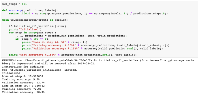
Look at this paragraph of code, first of all, it defined a utility function named “accuracy” which calculate the prediction accuracy based comparing the labels with the predictions. The prediction variable is the output from the softmax function which is, in essence, the probability of certain class happening out of all the possible classes.

For example, we have three classes (‘a’, ‘b’, ‘c’), the predicted logits could be

3.0, 1.0, 0.2

. And the corresponding softmax output (predictions) will be (refer to this stackoverflow question)

[ 0.8360188   0.11314284  0.05083836]

np.argmax function will return the index of the largest element.

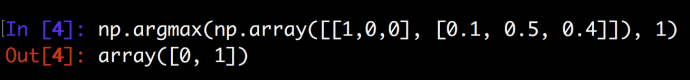
compare the maximum index of the prediction with the one for labels will give you the true / false at row level and you can easily calculate the overall accuracy then.

After that, they run 801 loops and each loop will calculate the loss function for all the data points and report out the accuracy every 100 records for easier readability.

As you can see, the implementation is so neat and clean which tensorflow packages all the variable updates behind the scene.

STOCHASTIC GRADIENT DESCENT

Now let’s look at the source code of the stochastic gradient descent. it is very much like the previous code and the only difference is every step/loop, we only feed a batch of data to the optimizer to calculate the loss function.

For example, the batch size here is 128 and the subset data set is 10,000. This should improve the loss function calculate by 80x faster. And instead of reusing the same data again and again, we will loop through all the training data in a batching way so in that case, we will gain the training performance gain and we used all the data points at least somewhere in our code. The overall accuracy was as good as plain gradient descent.

In the next post, we will try to solve the problem of improving this logistic regression and evolve into a neural network with hidden layers and other cool stuff.

“Turn the logistic regression example with SGD into a 1-hidden layer neural network with rectified linear units nn.relu() and 1024 hidden nodes. This model should improve your validation / test accuracy.”

Challenge Accepted!