In the previous post, we briefly covered how the iPython notebook read the pickled inputs and transformed into a workable format. Today, we are going to cover the following block of how to create an optimizer which will be used during the iterations.

GRAPH

Any tensorflow job could be represented by a graph, which is a combination of operations (computation) and tensors (data). There is always a default graph object got established to store everything. You can also explicitly create a graph like “g = tf.Graph()” and then you can use g everywhere to refer to that specific one. If you want to save the headache of worrying about switching between graphs, you can use the “with” statement and all the operations within that block will be saved to the graph handler.

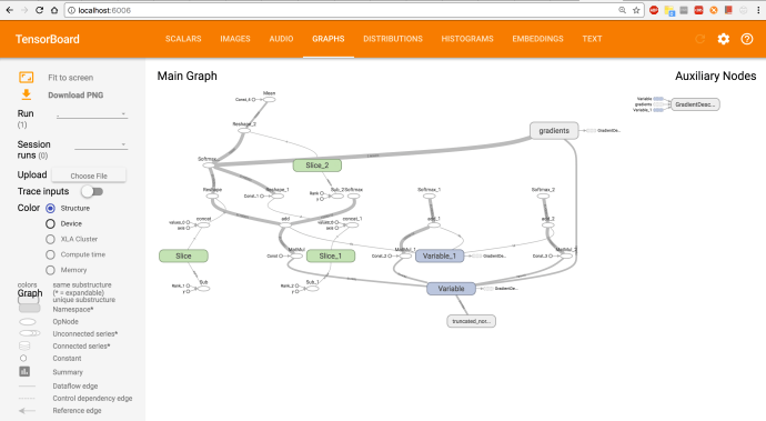
Also, “a picture is better than a thousand words”, there is a tool called tensorboard which is extremely easy to use to help you visualize and explore the tensorflow graph. In this case, I am simply adding extra two lines of code at the end of the graph with statement block.

The writer will write the graph to a file and writer.flush will ensure all the operations which got asynchronously written to the log file is flushed out to the disk.

Then you can open up your terminal and run tensorboard command:

$ tensorboard --logdir=~/Desktop/tensorflow/tensorflow/examples/udacity/tf_log/
Starting TensorBoard 47 at http://0.0.0.0:6006
(Press CTRL+C to quit)

And this is how it looks like that block of Python code.

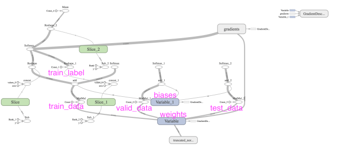
The labels on the tensorboard does not necessarily reflect how variables are named in your code. For example, we first created four constants, the true tensor name only shows up when you print out the four constants.

tf_train_dataset:  Tensor("Const:0", shape=(10000, 784), dtype=float32)
tf_train_labels Tensor("Const_1:0", shape=(10000, 10), dtype=float32)
tf_valid_dataset Tensor("Const_2:0", shape=(10000, 784), dtype=float32)
tf_test_dataset Tensor("Const_3:0", shape=(10000, 784), dtype=float32)

Then, it is also pretty cumbersome to map each variable to the corresponding unit in the graph. Here is how the graph looks like after I highlighted some of the key variables.

LOSS

The loss function or cost function for a deep learning network are usually adopting a cross entropy function. It is simply

C=−(1/n) ∑[y*ln(a)+(1−y)*ln(1−a)]

y is the expected outcome or label. In a one hot coding fashion, y is either 0 or 1 which simplified the C = -1/n * ∑ln(a), and here “a” is the predicted probability, which is the normalized outcome done by the softmax function. 

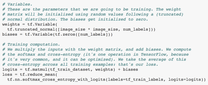
In this paragraph of code, it first created a variable weight of size (28*28~784, 10) and the bias variable of size (10). Weight was initialized by a normal distribution but throw away all the variables outside two standard deviation range while biases are initialized to be zero to get started. Just to recapture, our tf_train_dataset variable is now a N by 784 size matrix where N is the number of records/images the user specify.

logits = x * w + b = (N,784) * (784, 10) + (10) = (N, 10) + (10) = (N, 10)

Now logits is a matrix of N rows and 10 columns. Each row contains 10 numbers which store a unnormalized format of the “probability” of which hand written digits that record might be. The highest number definitely indicates the column/label it falls under is mostly likely to be the recognized digits, however, since all the numbers are simply the outcome after W*x+b which is necessary to be bounded to be between (0,1) and further more, they do not add up to 1. Those normalization all happens behind the scene in the nn.softmax_cross_entropy_with_logits function. As an end user, we only need to make sure we memorize what logits truly stands for and how you calculate logits. Tensorflow.nn will take care of the rest.

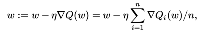
Optimizer

optimizer = tf.train.GradientDescentOptimizer(0.5).minimize(loss)
In this example, the author used the GradienDescentOptimizer. 0.5 is the learning rate.

 

# Predictions for the training, validation, and test data.
# These are not part of training, but merely here so that we can report
# accuracy figures as we train.
 train_prediction = tf.nn.softmax(logits)
 valid_prediction = tf.nn.softmax(tf.matmul(tf_valid_dataset, weights) + biases)
 test_prediction  = tf.nn.softmax(tf.matmul(tf_test_dataset, weights) + biases)

Last but not least, they called the softmax function on training/valid/testing dataset in order to calculate the predictions in order to measure the accuracy.

In the next post, we will see how tensorflow frame work will iterate through batches of training dataset and improve the accuracy as we learn.