This is a video that I took with startcraft II in ultra setting running in the Cloud thanks to Geforce NOW.

First, here are some “lowlights” of my gaming machine:

• CPU: Processor AMD FX(tm)-6120 Six-Core Processor, 3500 Mhz, 3 Core(s), 6 Logical Processor(s)
• GPU: GTX 1050ti (upgraded)
• Memory: 16 GB (upgraded)

Now, let’s get to my experience of how Geforce Now surprised me.

I came across an activation code in my email inbox that Nvidia actually granted me the access to the Geforce Now free beta. I decided to give it a try and it turned out the experience was fantastic. In essence, it is to off load your gaming machine from doing all the heavy computing, instead, run the game on Nvidia hosted virtual environment and of course, you have to have reasonable and stable network to get the full value of it.

My office is in the second floor and the router is on the first. The wireless internet connection is mediocre so this test isn’t really the best representation of the full capability of Geforce Now. I am tested Starcraft II, Diablo III and battleground and all three of them performed really well.

The lagging is minimized to the internet connection, for Starcraft II players like me who doesn’t have a 300 APM, that lagging is trivial and doesn’t now really impact the gaming experience, but I am assuming if you are playing with any competitive shooting game, that few ms might matter. Anything else should be perfectly fine. I even bought battleground on the fly because my computer was never capable of running it and now I can play it on the Cloud, I spent quite a few minutes just staring at the sky rendered by those crazy machines in the cloud.

I see this literally as a game changer because by pooling all the gaming computing power into one centralized place, this should theoretically drop the total costing of each household spend thousands of dollars on getting the best gear on their own. However, I don’t think a company is running a charity but to maximize their shareholder financial benefits. As an end consumer, I know that the internet is getting faster and better (like 5G), if Nvidia is asking me should I buy a gaming PC or use their service, I might be willing to pay the subscription to play Geforce Now if the monthly subscription fee is close or lower to the monthly depreciation of the hardware.

Say a gaming machine is $2,000 and you expect to get the full usage of it and replace in three years. 2000/3/12 ~ $55/month. Of course, you don’t buy computers only to play games but for many gamers, they do upgrade their gear only because of gaming performance. Also, take into consideration that you can unsubscribe if you are taking a long vacation or busy working, it pays back.

Anyway, good job to Nvidia as usual and this made me wonder if our next generation will be asking the question “hey, daddy, what is that big black box? shouldn’t everything run on a TV directly?” 🙂

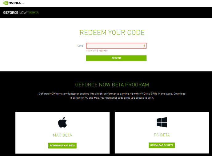
Download Geforce Now beta test

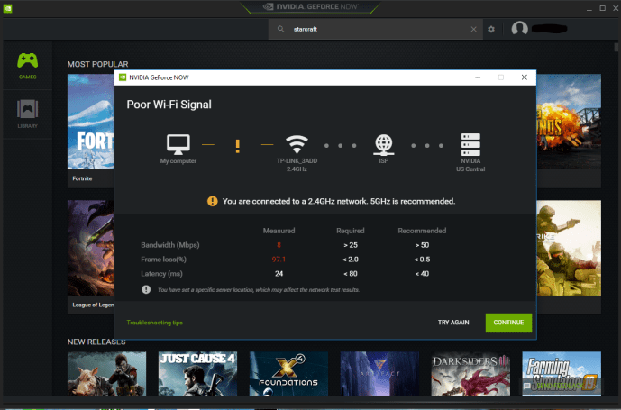
Run a test. My internet is on the low end and far from the router but still working.

Looks like from this step, it is already running on a Windows virtual machine. I am assuming they are collecting all the information like IP address, hardware spec in order to align the cloud resource to be best compatible with the consumer terminal.

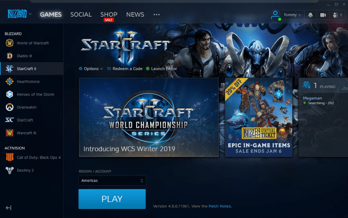
Works perfect for me.

You can easily enable Ubuntu to run as a subsystem in Windows 10.

Following the tutorial here to enable the subsystem and everything else is as easy a few clicks.

You can also access windows files from the linux file system.

After all, good luck.

This is a blog post to familiarize ourselves with the functions that we are going to use to calculate the cross correlation of stock prices. In this case, we are going to create some dummy time series data, one is the leading indicator for the other and hopefully pull the necessary strings to detect it and plot and understand it how it works in the Python realm.

1. time series

Time series data is the best representation of signals like temperature history, pricing history, inventory history, balance history and pretty much any kind of history used in day to day life. We can either use a pandas dataframe or actually, in this case, use the Series class and make the datetime field to be the index.

In this case, we generated a series of 8 elements starting at 2018/01/01. Then we are going to generate another series which is a leading indicator of 2 days ahead of s_a.

Before we hard code another series which is, say one day of ahead of the first series, like [0,0,1,2,3,2,1,0]. Let’s check out if there is any method of pd.Series that we can use. There is a whole lot of functions that can be used to time series data. And the closest function that might serve our purpose looks like shift, tshift, sliceshift.

shift method indeed looks very powerful where it cannot only shift to fix on the datetime window and shift the value away by filling in NA, but also, if required, will be able to shift the window by a specified frequency. The last print statement shows a perfect way to generate another leading indicator of s_a by two days.

After generating the leading indicator, we can put them side by side so that it is obvious to you. pd.concat is a really powerful function that I will dedicate another whole article to talk about but for now, it serves the purpose of doing a full outer join of those two time series data by date.

Cherry on top of the cake, this is the visualization of two signals with one 2 days of ahead of the other.

2. cross correlation

Cross correlation is to calculate the dot product for two series trying all the possible shiftings. For example, let’s fix the s_a and assume that you slide s_b from the left to the right. At the beginning, s_b is far away and there is no intersection at all.

1. First intersection, Then as we move s_b to the right, the first intersection will be the far right element of s_b cross the far left element of s_a. In this case [1] from s_b and [0] from s_a. And the dot product is 0. Hence, the first 0 in the corr variable.
2. Second intersection, it will the be two far right elements of s_b, [2,1] crosses the two far left elements of s_a [0,0], which still ends with a 0.
3. …
4. Actually, it is not until there are four elements intersect which is [0,0,0,1] and [2,3,2,1] where the dot product is 1.
5. so on and so forth till the far left element of s_b cross far right element of s_a.
6. Then s_a keep moving to the left and s_b moving to the right and they will never cross again.

As you see, in our dummy example, the dot product is maximized when these two list perfectly aligned with each other perfect vertically. However, here we are only aligning the values, let’s take a look at the index. In this case, we can pick at element in either list. The first 0 from s_a represent  2018-01-01 and the first 0 from s_b represent 2017-12-30. Now we know that s_b is 2 days ahead of s_a purely by analyzing the cross correlation and that is exactly how we constructed s_b in the first place, isn’t it?

In this case, we are simply calculating a sliding dot product which is not necessary the traditional correlation like pearson correlation, for example, how could a correlation be greater than 1, right? There is a good stackoverflow question that sort of addresses this problem.

We can see that the cross correlation is maximized at position 8th, and the length of both s_a and s_b are 8. so no doubt, the two series need to be perfectly aligned. Let’s take a look at another example when two series have different patterns and lengths.

The cross correlation is maximized when s_b is shifted to the right by 7 in this case, actually is when the maximum of s_b align with the maximum of s_a aligned.

3. summary

cross correlation is useful when you try to find a position (lagging/leading) when you compare two time series that doesn’t have to necessary share the same length.

(note: don’t confuse yourself with the pearson correlation, cross correlation doesn’t have to necessarily be between -1 and 1)

Seeing the dead end of paying out an API to query all the companies, I decided to give my luck a try. There must be some sites which has the beautiful csv file that I have been looking for somewhere on the internet. Don’t give up!

This post will be a quick documentation of how I found a public dataset about stock prices from Kaggle and most importantly, how to observe and get the data into a clean format in a database for later research.

1. Download

Frankly speaking, there are indeed so many places where you can possibly scrape the data off if you approach it carefully, at the same time, there are also data sets on Quandl / Quantopian where you still have to be a premium user in order to use it. However, after some research, Kaggle – this community where data analysts/developers banging their heads against difficult machine learning problems indeed has the solution for me.

They a datasets repositary where some really cool data were published in public. After a quick search, you can find several datasets related to equity prices and some even with the financial performance for those companies, the fundamentals, that we can play with later, for now, our focus will be the “Huge Stock Market Dataset”

2. Extraction

The data has a decent size and I will kindly warn those windows users who uses the default compression/decompression program, it will be slow for you. I have a pretty old HP desktop and it was decompressing the file at a ~1MB/s speed, that will take me tons of time. I highly recommend 7zip which is a free archive application that can totally deals with commonly use compression format. And for me, it was 5 times speed time.

3. Format

First, let’s take a quick look at the dataset. The uncompressed format is about ~770MB that has 8500 files. It is categorized into two folders, the ETF and the Stock:

The data is structured in such a way where each symbol/ticker is a individual text file on its own, and all following the format of symbol.us.txt format.

Let’s take a look at Apple’s data file to understand the file structure.

It looks like a pretty classic CSV (common separated file) contains the daily prices since 1984-09-07. It indeed goes back a long time but Apple issued its IPO on December 1980 so I don’t think this dataset contains all the history. Another quick check is to understand if the stock price has been adjusted, in a way where whenever there is a stock merge/split, the price is baselined or normalized for analysis purpose. If not, our analysis might take the risk of reaching to the conclusion where the stock price dropped by 50% which in fact, it is merely a 2-1 split.

By visiting Apple’s website, you know they have issued stock split 4 times, 1 time for a 7-1 split and the rest is 2-1.

So theoretically, one stock at IPO is now equivalent to 1 * 2 * 2 * 2 * 7 = 56 stocks of today. I came across a blog post from Maria Langer and the story that she shared how she her stocks grew since 1997 is totally interesting and inspiring. In the end, I did find a picture of a 1998 Apple stock certificate to show you how expense those stocks could be today if there was not stock split.

This certificate was issued at Apr, 30, 1998. And there are there has been three split (2*2*7=28) since then. By the market close this Friday, each stock is ~ $165. So if there has never been stock split, you need will need a lump sum of $4620 to just buy one Apple stock. That will totally change the demographics of the investor for Apple, probably only high net wealth individual or institutions will be able to invest, much less liquidity and probably won’t be as successfully as it is today as a house hold name.

Anyhow, like Yahoo finance, its pricing data is adjusted in a way taken stock split into consideration.

The Apple was IPOed at $22 per share. And in Yahoo Finance, the Dec 1980 price was $0.51, which aligns with the stock split. ($0.51 * 56=$28 ~ $22). People might say “should have I invested $XXX, I would have $YYY today”, the short answer is even if you were an investor at that time, 1980s, it was actually very difficult to see companies like Apple to be a good company to invest.

All those hyper growth looks exciting but let’s compare it with the interest rate. For example, the Fed Interest rate in 1980 was 17.26%. By the time this blog was written, the FED rate is only between 2~3%. If the risk free rate was that high, I really couldn’t imagine how could anyone take the risk and invest their savings into a tech startup with the their CEO dress like college students.

To prove my point, you can pull the FED rate and the risk free holding period return is 523% if you buy T-bill.

That is a mouthful and enough distraction, let’s get back to see if our dataset actually contains the adjusted price. Clearly, the starting price is 42 cents which is far less than $22 in 1984. It is a good indicator that the data downloaded is adjusted.

 4. ETL – Database

Even if the data is already in text format and on your disk, my personal preference is to convert that into a format that is easier to deal with like to put into a database. For now, let’s dump it into SQLite. Then, it will be pretty easy to do some analytics or connect with other tools like Python and visualizations tools more easily.

By using Pandas and SQLalchemy, the life now is so easy. Since this conversion requires a lot of disk read and write, it took me a while, about half an hour, so it is a good idea to add in a progress bar and try except logic.

In the end, we ended up with 32 companies somehow got empty file in the txt file which are

['accp', 'amrh', 'amrhw', 'asns', 'bbrx', 'bolt', 'boxl', 'bxg', 'ehr', 'fmax', 'gnst', 'hayu', 'jt', 'mapi', 'molc', 'otg', 'pbio', 'pxus', 'rbio', 'sail', 'sbt', 'scci', 'scph', 'send', 'sfix', 'srva', 'stnl', 'vist', 'vmet', 'wnfm', 'wspt', 'znwaa']

I took a quick look at the Yahoo finance and they do look legit companies some with good history of data, but I guess we will put a pin the question of why they are missing data and focus on the ones that we have.

After all of this, 17 million records for 8507 different public companies (a count distinct took 45 seconds without indexing so be cautious when you play with complex queries) and database is about 1.3 GB.

In the next post, we will do some descriptive analytics and hopefully figure out an efficient way of manipulating the data.

If you are interested in playing with time series data like stock price, it is usually a good idea to start with Finance, probably the most frequently used exchange stock price. There are many exchanges out there and NASDAQ is a good one. I shopped around on the Internet but it is a bit hard to find some good dataset with fine grained data without paying. However, there are plenty of free APIs out there but they are all based on tickers so in this case, we can put together a solution where we can first get a list of public company names and then loop through each company but making an API call each specifying the time range.

1. Get Company List

By visiting Nasdaq website, you can easily find a download file which contains all the tickers that listed there (not only Nasdaq but also Amex and NYSE).

And this is how the data file looks like.

This is the first time I ever see 3435 public companies listed in such a clean format, let’s do some quick analysis. Since the industry is a subcategory of Sector and have if not hundreds, at least tens of different categories that might be difficult to display. For now, let’s aggregate by sector and see what are the total market cap, number of companies, and maybe how “young” each sector is by calculating the median IPO year.

As you can see, technology sector has the most market cap (5.9trillion usd) which is almost half (46%) of the whole market. And the whole Nasdaq total market share is about ~ 13 trillion USD. At the same time, it is interesting to find that it is actually the finance industry who has the highest average IPO year and not surprisingly, consumer durables have the lowest/oldest average IPO year. From the company count perspective, Health care has the most number of public companies.

Anyway, now we have a trustworthy list of tickers, the next step is to hit the API and get the time series stock price for those companies via alpha vantage.

2. Get Time Series data

I put together this little program so that I can make calls and then store the raw response to my local disk for later processing. Sqlite is a good option and you can use dbbrowser to view the table content easily.

One small tip is that the insert statement above is an easy way to escape all the characters by using the question mark placeholder. Quite neat so that you don’t have to play with double quotes and single quotes, which is a big pain in the ass.

Unfortunately, my job couldn’t finish even for my tests against just the first 10 companies, and I should have guess it way ahead of time, it is a “free-mium” service, the API has an extremely small limit which if you are trying to make more than 5 calls in a minute, you need to upgrade to the premium services, which I am not fully ready to do that yet. I guess this is the end of post. A perfect example how difficult and time consuming it could be to hunt down the good data sources.

Frankly speaking, it is indeed not that expensive but I guess as a hobbyist, you probably want to shop around and see if there is a better choice for your weekend project.