Best First Tree Builder

In the _tree.pyx file, there is a very interesting implementation of a type of TreeBuilder called the BestFirstTreeBuilder. The __cinit__ is very boilerplate but all the intelligence actually sits in the build method.

In the BestFirstTreeBuilder, they used the data structure PriorityHeap to implement the priority binary tree. There are two key variables, the max_split_nodes and max_leaf_nodes which are being used to declare the initial capacity.

Screen Shot 2019-10-27 at 9.52.43 AM

In a complete binary tree, if root is at the depth 0, then at depth n, you will have 2^(n) total leaves at the bottom of the tree. And all the nodes above will be split nodes. And in total, you will have 1+2+4 … = 2^0 + 2^1 + 2^2 + … + 2^(n-1) = 2^n – 1. That is why max_split_nodes = max_leaf_nodes – 1 and initial capacity is the sum of those two. Screen Shot 2019-10-27 at 9.58.24 AM

Then the rest of the build method will recursively build the tree following the “priority”.

Screen Shot 2019-10-27 at 10.10.30 AM

There are two methods which we will cover here. self._add_split_node will compute the split node and _add_to_frontier will add the split to the frontier.


Pickle

Here is a bit more about the Pickle and how you can customize how the pickling process work, use __getstate__ to customize how things got pickle.dumps and use __setstate__ to customize how things got pickle.loads.

It is not recommended but you can also use __reduce__ if you know what you are doing.

__getstate__ and __setstate__

Screen Shot 2019-10-27 at 11.00.40 PM

__reduce__

Screen Shot 2019-10-27 at 11.18.30 PM

cdef class Tree

Array-based representation of a binary decision tree.
    The binary tree is represented as a number of parallel arrays. The i-th
    element of each array holds information about the node `i`. Node 0 is the
    tree’s root. You can find a detailed description of all arrays in
    `_tree.pxd`. NOTE: Some of the arrays only apply to either leaves or split
    nodes, resp. In this case the values of nodes of the other type are
    arbitrary!

For a tree, it certainly has a few non-array attributes like node_count, capacity and max_depth. Other than those three, there are 8 methods which are arrays and all unanimously has the size of node_count.

1. children_left

each element stores the node id of the left children for the i-th node, of course, if i-th node doesn’t any child, it will use the value TREE_LEAF=-1.   As the binary tree always follow the priority that the left child will always has the values that smaller than the threshold. Of course, all the children have a node id greater than its direct split node so children_left[i] > i.

2. children_right

very similar to child_left

3. feature

feature[i] holds the feature to split on for the internal node i -> Key

4. threshold

threshold[i] holds the threshold for the internal node i -> Value

5. value

value is a bit complex, it has the shape of [node_count, n_outputs, max_n_classes]. The documentation says “Contains the constant prediction value of each node.

6. impurity:

impurity at node i

7. n_node_samples:

holds the number of training samples reaching node i

8. weighted_n_node_samples:

holds the weighted number of training samples reaching node i
Screen Shot 2019-10-27 at 5.06.52 PMScreen Shot 2019-10-27 at 5.13.23 PM
In the tree method, there are not that many methods that meant to be used by the users, and the sklearn developers achieved this goal by forcing the methods to be only available in Cython by declaring them using cdef. However, there are still a few methods that are being defined using cpdef which must be familiar to most sklearn users.
1. predict(X)
Screen Shot 2019-10-27 at 8.38.47 PM
2. apply(X)
Screen Shot 2019-10-27 at 5.25.46 PM
3. decision_path(X)
The decision_path code is very similar to other methods which it look through all the samples, and within each sample, it will populate the outcome. However, within the code of decision_path, it has used the indptr and indices and also the pointer to these two arrays, indptr_ptr and indices_ptr to point to the data.
Screen Shot 2019-10-27 at 8.56.10 PM
If you are confused by indices, indptr and data, don’t worry, all those variables are the key variables for the CSR (compressed sparse rows) matrix in Scipy.
Instead of reading its official documentation, you can find this great Stackoverflow question. Here is a screenshot provided by user Tanguy explaining how those variables got put together.
csr.png
4. compute_feature_importances()
Screen Shot 2019-10-27 at 5.17.53 PM

SKLEARN SOURCE CODE TREE – PART II

This post dives into the sklearn decision tree building process.

The node_split method within the BestSplitter class is probably the most element implementation that I will say within the whole decision tree module. Not only it entails the implementation of the splitting process, but also demonstrated a myriad of core computer science concepts. Now let’s go through these 200 LOC and enjoy.

Screen Shot 2019-10-14 at 11.30.47 PM

In the method documentation string, it is mean to “Find the best split on node samples[start:end]”. Variable samples store all the samples, or each node_split is not necessarily running against the whole samples at every split. During each split, its range will target at the start:end range which will find the rotation later.

Meanwhile, at each node_split, its inputs include not only the latest impurity process, it also contains a pointer split to the split record, last but not least, for efficiency purpose, the splitters keep track of the number of constant_features so we can speed up the splitting by avoiding constant features, hence the comments below:

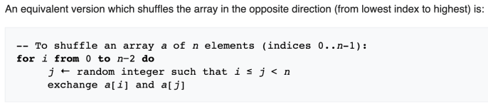
        # Sample up to max_features without replacement using a
        # Fisher-Yates-based algorithm (using the local variables `f_i` and
        # `f_j` to compute a permutation of the `features` array).
        #
        # Skip the CPU intensive evaluation of the impurity criterion for
        # features that were already detected as constant (hence not suitable
        # for good splitting) by ancestor nodes and save the information on
        # newly discovered constant features to spare computation on descendant
        # nodes.

First, let’s look at the outermost loop and its condition:

  1. f_i > n_total_constants
  2. n_visited_features < max_features
  3. n_visited_features <= n_found_constants + n_drawn_constants

condition 1 and (condition 2 or condition 3)

max_features is a an input variable that can be changed by the user, but default to be the total number of features. When float, it will analyze pick a fraction of all the features during the split or hard coded to be a specific number of features.

The implementation takes into account constant variables, and has several flags/counter to keep track in order to improve the performance. However, that might not help the reader so we will assume all the columns are not constant so any counter related to constant will be zero.

In that case, the while loop condition will be (f_i > 0 and n_visited_features < max).

n_visited_features is initialized to be zero and increases by 1 at each loop.

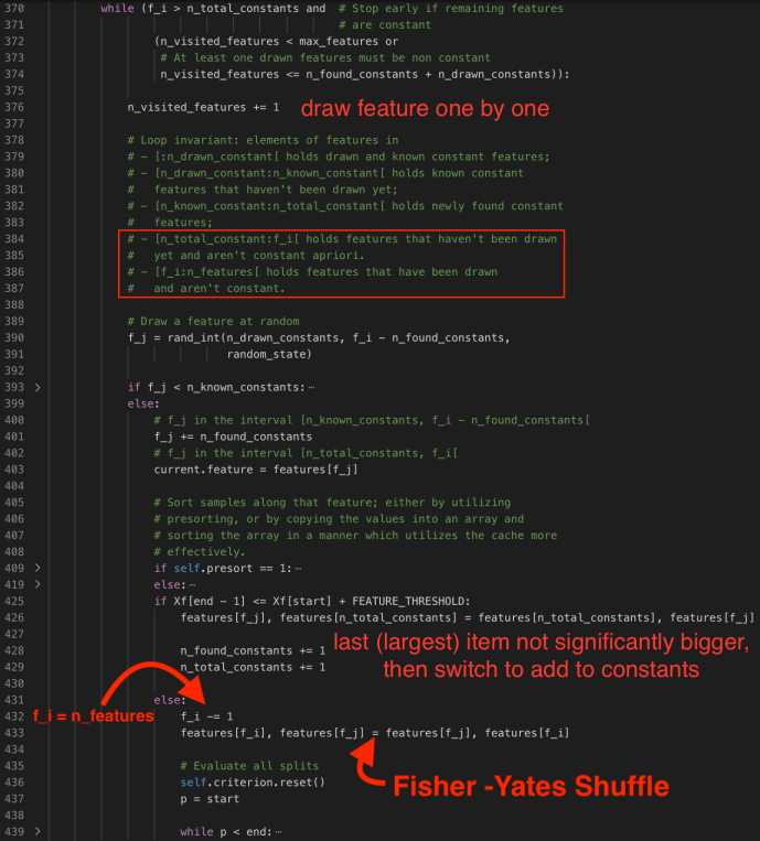
f_i was initialized to be n_features outside the loop, and at each loop f_j is randomly drawn from (n_drawn_constant, f_i – n_found_constants) ~ (0, f_i) when there is no constants. Of course, if we do have constants, f_j is meant to randomly select a feature that is not drawn nor not found constant.

When you draw the feature, the code checks what kind of feature this is, and update the related counter accordingly.

For example, as it is random sample without replacement, if it has been drawn, then it should not be drawn again, hence, f_j has to a random integer greater than the n_drawn_constants. f_j > n_drawn_constant.

At the same time, if f_j is smaller than n_known_constants, which means that we might have already known it is a constant without drawn yet (cache), then, we will mark this constant column as a drawn column by switch columns, append to the end of the drawn_constants range and update the n_drawn_constant counter by one.

Of course, we don’t know yet, we will update f_j by adding the identified/found constants so f_j is now pointing to the f_j th unidentified column and use it as the current feature.

Once we select a feature, then we will copy the column values to a new array Xf and sort the values. After we sort the values, then we will check to see if the column is close enough to be constant by comparing the min Xf[start] and max Xf[end-1] and see if the difference is smaller than feature_threshold. If so, of course, we will update the found_constants by 1 and total_constant by 1.

Of course, after all, if is not known constants, or if it is new but not constant, then we will go and find the split points by decreasing f_i by 1 and switch values of feature f_i and f_j. In that case, our randomly selected features will always be at the end of the list and slowly building up to the start of the queue.

Screen Shot 2019-10-14 at 10.55.54 PMScreen Shot 2019-10-14 at 11.10.55 PM

When the feature is properly sampled, they first initialize the position – variable p to be the start, the record index of the first sample. And it will go through each record. In addition, when it moves on to the next record, they FEATURE_THRESHOLD to make sure that it was not numerically equal, if so, they will skip to the next record which is materially different.

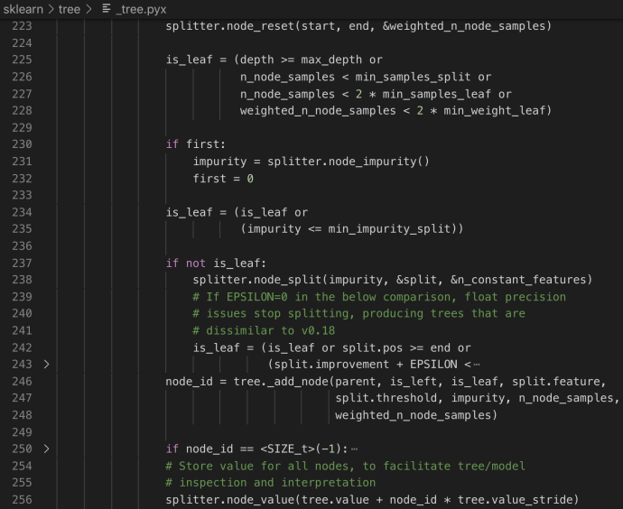
When sklearn is trying to find a split point during a continuous range, there is a very important user input called min_samples_leaf, which is defaulted to 1. When you build a decision tree, theoretically, you can train your model to be 100% accuracy during the training stage by creating a tree path which each unique record falls into its own path. Your model will for sure be big, and at the same time, you might be cursed with overfitting your data that during the prediction stage, the accuracy will be drastically lower. To avoid that, min_samples_leaf can be used to make sure you only create split point when the children has more than min_samples_leaf data. Here is the official documentation.

Screen Shot 2019-10-26 at 10.38.57 PM

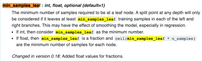
The same idea applies to the min_weight_leaf in which instead of samples count, the requirements hold true for sum of weight.

After these two checks, they will calculate the criterion improvement and calculate with the record keeper until they loop through all positions and find the best split point and save that position as the best.

Screen Shot 2019-10-14 at 10.39.45 PM

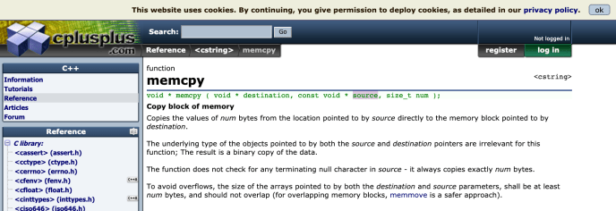
After they find the best split point, they will “Reorganize” and actually split the samples using the best split point. Keep in mind that X still holds the raw samples and are NOT sorted. while p:= start < partition_end := end is an interesting way of splitting the data and sort into two subgroups in which left part of the array are always smaller and the right is always larger.

Here is a small Python script to demonstrate how it works, just to clarify, the data is still not completely sorted.

Screen Shot 2019-10-26 at 11.05.31 PM.png

Screen Shot 2019-10-14 at 11.19.24 PM

After the “Reorganization”, the memory of constant features will be copied and return the best split point.

Screen Shot 2019-10-26 at 11.15.35 PM.png

In summary, in this post, we have covered the split_node method with in the BestSplitter class. We looked at how they use Fisher_Yates random sample the features, for a given feature, how it find the best splitting point and at last, how it cleaned everything up and pass on to the children.


sklearn Source Code tree – Part I

This post, actually this upcoming series of posts, will be focused on gaining more knowledge of the exactly implementation of sklearn. Not only how in depth the algorithm got implemented, but also learning the best practices and styles of one of the most popular python library or even machine learning library out there. And today focus will be looking at the _tree.pyx.

To really dive into the details of trees, one has to be familiar with the underlying data structure used for implementing a decision tree, or a tree in general. Under the _utils.pxd, can you easily find the declarations for two key data structures Stack and Priority Heap and its relevant implementation atomic unit – StackRecord and PriorityHeapRecord.

Screen Shot 2019-10-13 at 9.59.39 PM

No surprise, Stack is the commonly used data structure which supports FILO logic, hence, we have the push and pop method. Each record is actually fairly interesting which we are going to future explain what each attribute is being used for.

After that, it is another data structure called priorityHeap.

Screen Shot 2019-10-13 at 10.07.12 PM

I came across a great post about PriorityQueue with BinaryHeap which you can find the more interesting reading and Python implementation here. At a very high level, the regular Stack is used for depth first tree builder and the PriorityHeap is used for the best first tree builder. In the ideal world, both tree builders will lead to the same final tree but one is learning faster and usually is preferred when we need cut off the learning process early with pruning (like decision stumps in GBM). To simplify, we will start by focusing on depth first tree builder.

Now let’s switch our eyeballs to the _tree.pxd.

Like StackRecord, the atomic unit of a tree is node, and each node is made of its left and right child (identified by the ID), the split feature, the threshold (regression), impurity gain during split, and others.

Then let’s take a look at the Tree class’es attributes. Node* and double* are the two pointers/arrays that store the true content of a decision tree.

Screen Shot 2019-10-13 at 10.23.34 PM

Now we have skimmed through the basic data structures, let’s switch to the _tree.pyx implementation and take a look.

Screen Shot 2019-10-13 at 10.42.51 PM

The whole _tree.pyx isn’t quite complex, only ~1600 LOC and if we are only interested in the Tree class implementation and the easiest tree builder DepthFirstTreeBuilder, you only need to read a few hundreds of lines of code. So let’s get started.

At the beginning, they first declared a TreeBuilder class as the basic interface which further got extended into different types of TreeBuilder (depth first or best first). It only has an internal method _check_input to ensure the data is contiguous.

Screen Shot 2019-10-13 at 10.29.41 PM.png

Across the whole implementation, there are numerous places that for performance reasons making calls to compress sparse matrix and others. Those functions play a pivotal role regarding making a python library fast enough but itself might deserve a dedicated series and less relevant to the tree implementation which we will skip for now.

Screen Shot 2019-10-13 at 10.51.05 PM
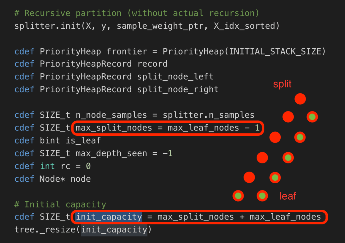
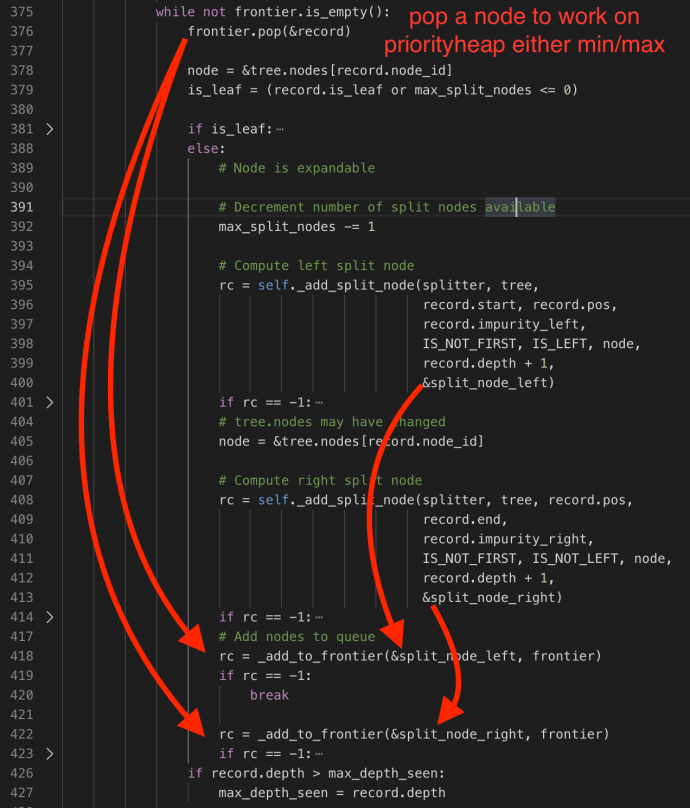
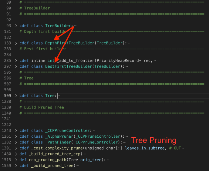
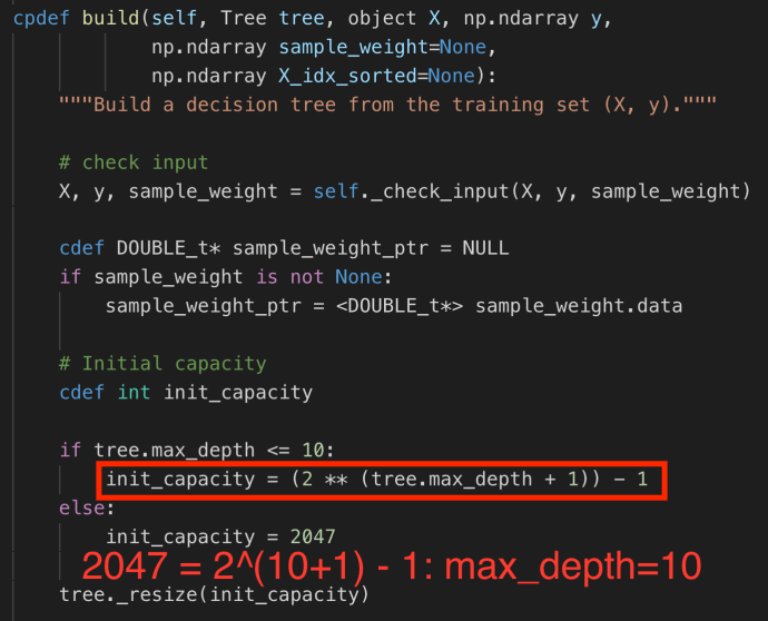
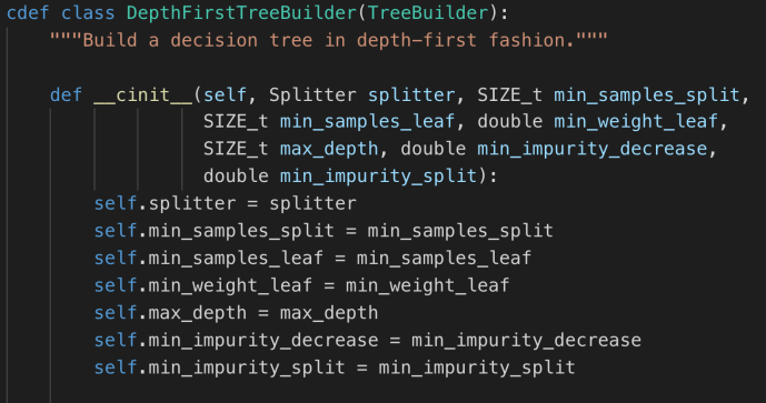
The constructor of DepthFirstTreeBuilder includes several key parameters when builder a tree. Splitter is the various splitter implementation which we will cover later. Now let’s go through the build method and see how each attribute drives the building process.

max_depth determines the maximum depth of the decision tree. As decision is a binary tree, when it is complete, the number of nodes grow exponentially. For example if you have 1 level, there are total 1 node, which is the root, if you have 2 levels, you have 3 nodes, and if you have three levels, you have 7 nodes, and when you have N levels, you will need 1+2+4+… = 2^0 + 2^1 + 2^2 + ..  2^ (N-1) = 2^N – 1 in total.

And as you can tell from the first few steps of the build method, that is exactly how max_depth is being used. Screen Shot 2019-10-13 at 10.56.29 PM.png

The next steps will be actually building the tree by working on the popped record and pushing its two children iteratively.

Screen Shot 2019-10-13 at 11.07.57 PM

As you can tell from the code, the stack will pop each record and replace with two children if any. And that is also the reason that why the stack has the size of INITIAL_STACK_SIZE which is 10, the same as the depth of the initial tree capacity. In this way, it will first build/traverse the left most branch and then bottom up, slowly transition to the right and traverse the whole tree with only a stack of 10 records. 

Now, let’s take a look at how splitter got called in the depth first tree building process.

Screen Shot 2019-10-13 at 11.36.10 PM

In the next post, we will spend more time looking into the node_split method and tree._add_node method to further understand the tree building details.