After we spent the previous few posts looking into decision trees, now is the time to see a few powerful ensemble methods built on top of decision trees. One of the most applicable ones is the gradient boosting tree. You can read more about ensemble from the sklearn ensemble user guide., this post will focus on reading the source code of gradient boosting implementation which is based at sklearn.ensemble._gb.py.
As introduced in the file docstring.
Gradient Boosted Regression Trees
This module contains methods for fitting gradient boosted regression trees for
both classification and regression.
The module structure is the following:
– The “BaseGradientBoosting“ base class implements a common “fit“ method
for all the estimators in the module. Regression and classification
only differ in the concrete “LossFunction“ used.
– “GradientBoostingClassifier“ implements gradient boosting for
classification problems.
– “GradientBoostingRegressor“ implements gradient boosting for
regression problems.
Almost the first thousand lines of code are all deprecated loss functions which got moved to the _gb_losses.py, which we can skip for now.
So let’s start by reading the BaseGradientBoosting class. The very majority of the inputs/attributes to BaseGradientBoosting are inputs to the decision tree also, and the ones that are not present in the BaseDecisionTree are actually the key elements for understanding GradientBoosting.
Now let’s take a look at the methods too.
__check_params is the basic checker to make sure the inputs/attributes are within the reasonable range and raise error if not.
__init_state, _clear_state, _resize_state and _is_initialized are all related to the lifecycle of states. One thing to watch out is that there are three key data structures to store the state, “estimators”, “train_score” and “oob (out of bag) improvements”. They all have the same number of rows as the number of estimators in which each row stores the metrics related to each estimator, and for the “estimators_”, each column stores the state for that particular class.
All the methods except “fit”, “apply” and “feature_importance” are intended as internal methods not being used by the end-users, hence, prefixed by a single underscore.
apply
Apply trees in the ensemble to X, return leaf indices
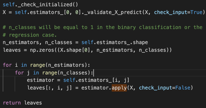
_validate_X_predict is the internal method for the class BaseDecisionTree which checks the data types and shapes, ensure they are compatible. Then we create an ndarray – leaves that of have as many elements as the number of input data. For each input row, there will also as many any elements as the estimators that we have established, finally, for each estimator, we will have as many classes as the prediction.
The double for loop here is basically to iterate through all the estimators and all the classes and populate the leaves variable using the apply method for the underlying estimator.
feature_importance
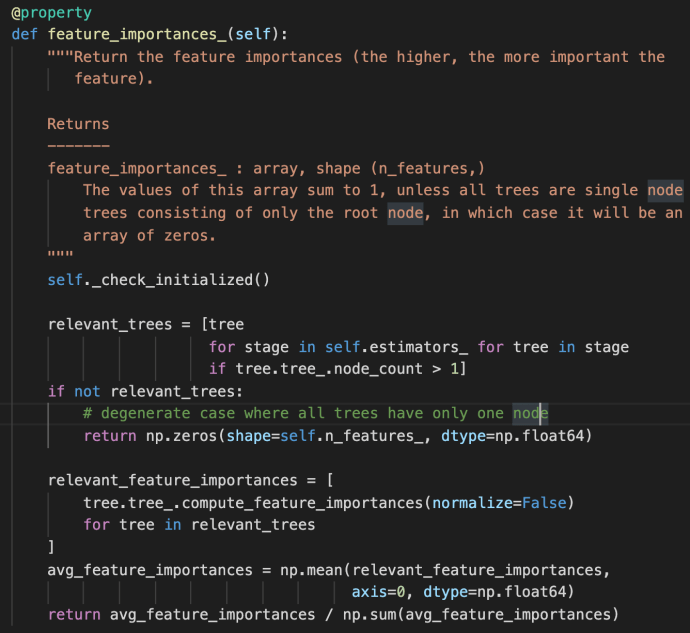
The feature_importances_ method first use a double for loop list comprehension to iterate through all the estimators and all the trees built within each stage. This is the very first time the term “stage” got introduced probably in this post. However, we have covered very briefly of the estimators_ attribute above in which each element represent one estimator. Then we can easily draw the conclusion that each stage is sort of representative of one estimator. In fact, that is how boosting works as indicated in the user guide –
“The train error at each iteration is stored in the train_score_ attribute of the gradient boosting model. The test error at each iterations can be obtained via the staged_predict method which returns a generator that yields the predictions at each stage. Plots like these can be used to determine the optimal number of trees (i.e. n_estimators) by early stopping. The plot on the right shows the feature importances which can be obtained via the feature_importances_ property.”
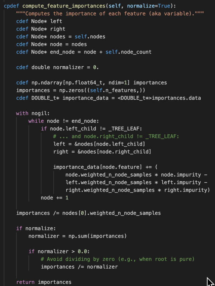
It is then literally the algorithmic average for the feature importance across all the relevant trees. Just as a friendly reminder, the compute_feature_importance method appear at the _tree.pyx method which is as below:
fit
“fit” method is THE most important method of the _gb.py, as it is calling lots of other internal methods which we will first introduce two short methods before we dive into its own implementation:
_raw_predict_init and _raw_predict
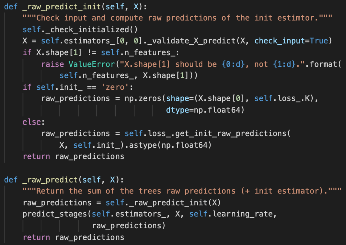
These methods are used jointly to generate the raw predictions given inputs matrix X and the returned value is also a matrix of shape that has the same number of rows as the input matrix and the same number of columns as the class types. The idea is very simple but this part is the core of the boosting process as boosting in nature is this constant iterations of doing predictions, calculate error, correct it and then doing this again. Hence, the predict_stages are implemented in high performance Cython.
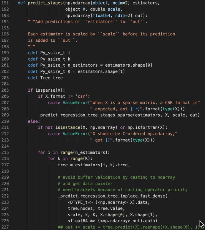
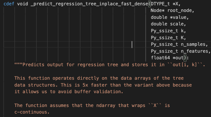
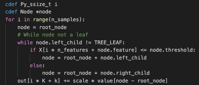
predict_stages iterate through all the estimators and all the classes and generate the predictions from the tree. This part of the code probably will deserve its own post explaining but let’s put a pin here and stop at these Cython code knowing that there is something complex going on here doing some predictions “really fast”.
fit
The fit method starts by checking the inputs of the X and ys. After that, it has some logic carving out the validation set which is driven by a technique called stratify.
You can find more about stratify or cross validation from this Stackoverflow question or the user guide directly. Meanwhile, knowing gd.fit has some mechanism of splitting the data is all you need to understand the following code.
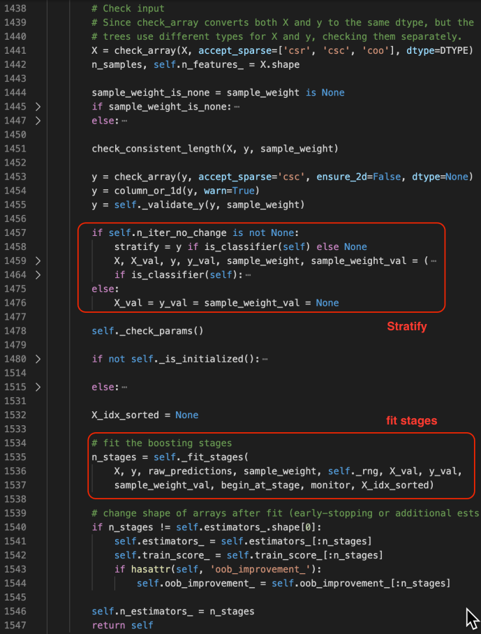
_fit_stages

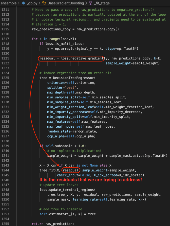
_fit_stage
Gradient Boosting Classifier and Regressor
After the BaseGradientBoosting class got introduced, they extend it slightly to the classifier and regressor which the end-user can utilize directly.
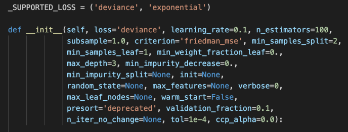
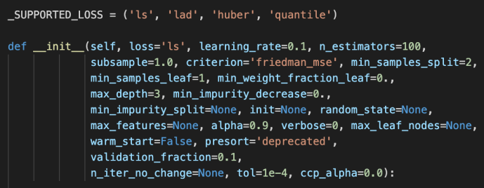
The main difference between these two is the loss functions being used. For regressor, it is the ls, lad, huber or quantile while the loss function for the classifier is the deviance or exponential loss functions.
Now, we can covered pretty much the whole _gb.py which we covered the how the relevant classes related to gradientboosting got implemented and at the same time owed a great amount of technical debt which I list here for few deeper dives in case the readers are interested.
- loss functions
- cross validation – stratify
- Cython in place predict