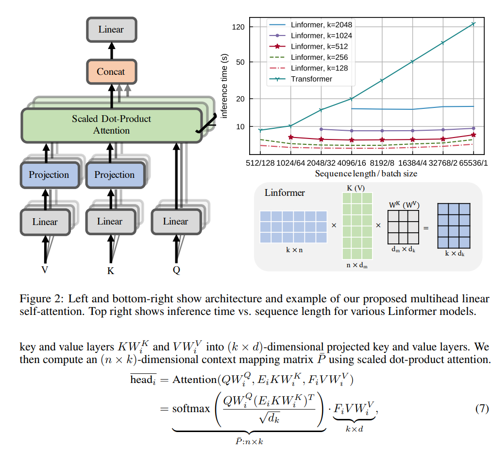
transformer has been commonly used in recommendation system and it is the key building block to model sequence. however, transformer is very expensive. the computational cost of transformer is n^2 * d + n * d^2, where n represents the sequence length, for social media platform, it is easy build a sequence with potentially hundreds of actions, so a sequence of length 1K immediately will turn into a 1M operations.
Where this 1M comes from is during the self attention when calculating the attention scores QK_t.
Q: n * d, K: n * d => Q @ K_t = (n * d) @ (n * d)T = n ^ 2.
To avoid this from happening, researchers found that matrix are low rank matrices, which means by dimension reduction, we can project these matrices smaller matrices that will have a fixed dimension of r instead of n.
In this psuedo code, we notice the attention score matrix is now n by r that grow linear with the sequence. In the very end, when we multiple with the value matrix, the dimension of r cancels out and we keep the final output exactly the same as the vanilla matrix. If we pick r to be 100 when n = 1000, using linformer will reduce the computation complexity by 10x.
Here are the study notes when I took the inference class from stanford cs336, discussing techniques to improve the inference efficiency.
Multi Head Attention MHA Grouped Head Attention GHA (use few keys and values) Multi Query Attention MQA Multi Head Latent Attention MLA (compressed latent KV): deepseek reduce N*H from 16348 to 512 MLA is not compatible with ROPE
Cross Layer Attention (CLA): reuse the same K, V projection between different layers
Local Attention full n^2 attention, sliding window attention, dilated sliding window, global+sliding window sliding window attention: KV cache size remain constant as you increase longer sequence size solution: interleave local attention with global attention (hybrid layers): for every 6 layers you have global attention
inference is memory limited – lower dimensional KV cache (GQA, MLA, shared KV cache) – local attention on some of the layers
alternative to transformers – state space models -> continuous state space, fast discrete representations – diffusion models – mamba – jamba: interleave Transformers and Mamba layers: 1:7 ratio – BASED: use linear attention + local attention – MiniMax: use linear attention + full attention (once in a while) (456 parameter MoE)
quantization: reduce precision of numbers, need to worry about accuracy fp32 4bytes: needed for parameters and optimizers states during training bf16: default for inference int8: for inference only LLM.int8()
model pruning
speculative decoding and speculative sampling: small model generation + big model evaluation is faster than big model generation, you get a 2x speedup, try to make draft model as close to the target model (model distillation)
I tested it on my local Ubuntu (I have windows and Ubuntu dual boot) and it worked great right off the shelf!
1. Installation.
installation of vllm is as easy as a pip install. because the inference is highly hardware dependent, depends on your hardware, you need to find the proper installation guide whether you have a nvidia card, a AMD card, a TPU, CPU etc. Sometimes, you even need to build from source directly to ensure the proper installation and best performance.
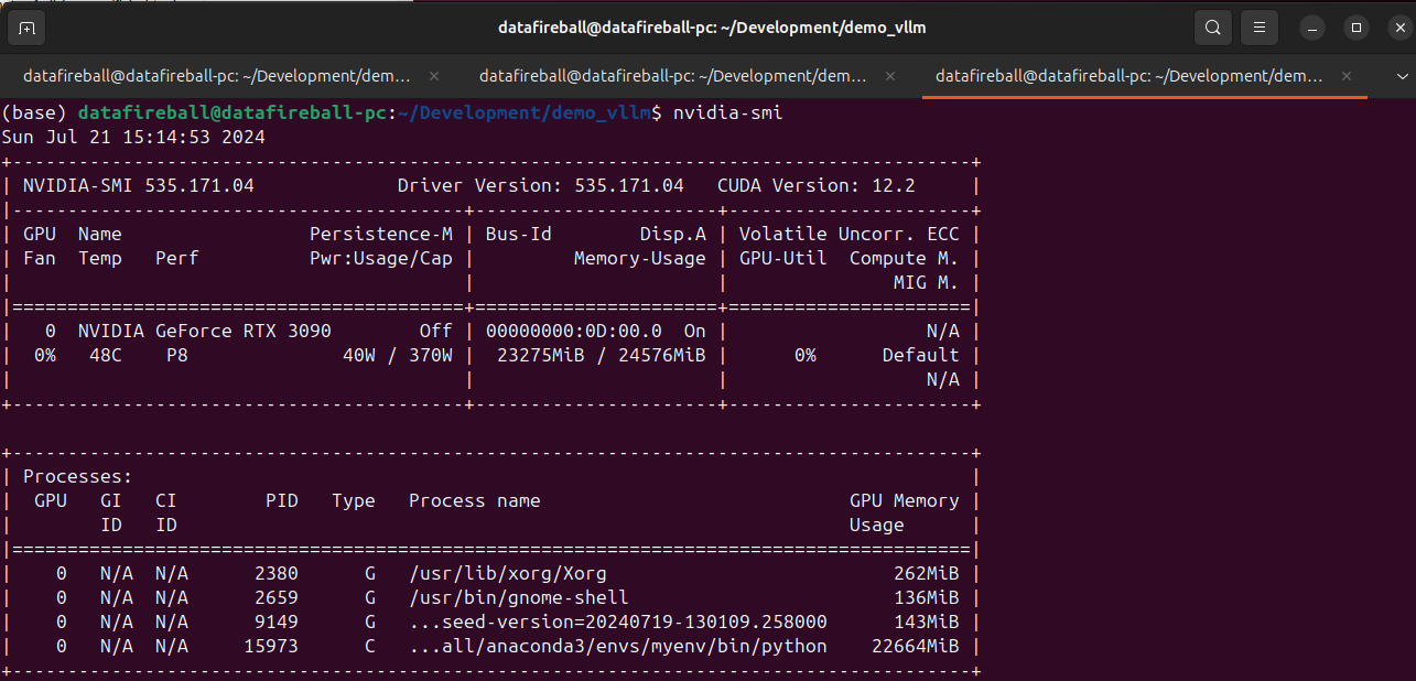
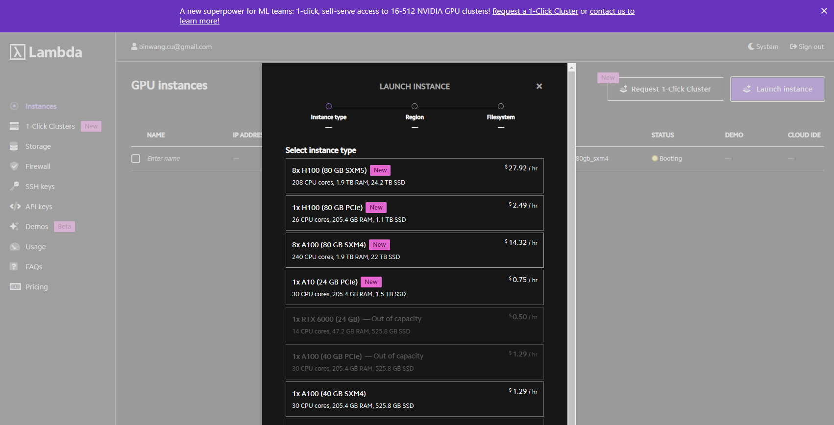
2. Check VRAM and GPU
make sure you have sufficient VRAM to host the model. Here I have a 3090 with 24GB VRAM.
3. Download the model and Serve
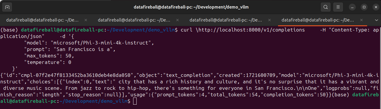
vllm supports many SOTA models, here is a list of all the models that they support. I am testing phi3 microsoft/Phi-3-mini-4k-instruct which is small enough to set up locally. Meanwhile, by downloading the instruct model, I can later refer it within within the gradio chat window to explore the chat experience.
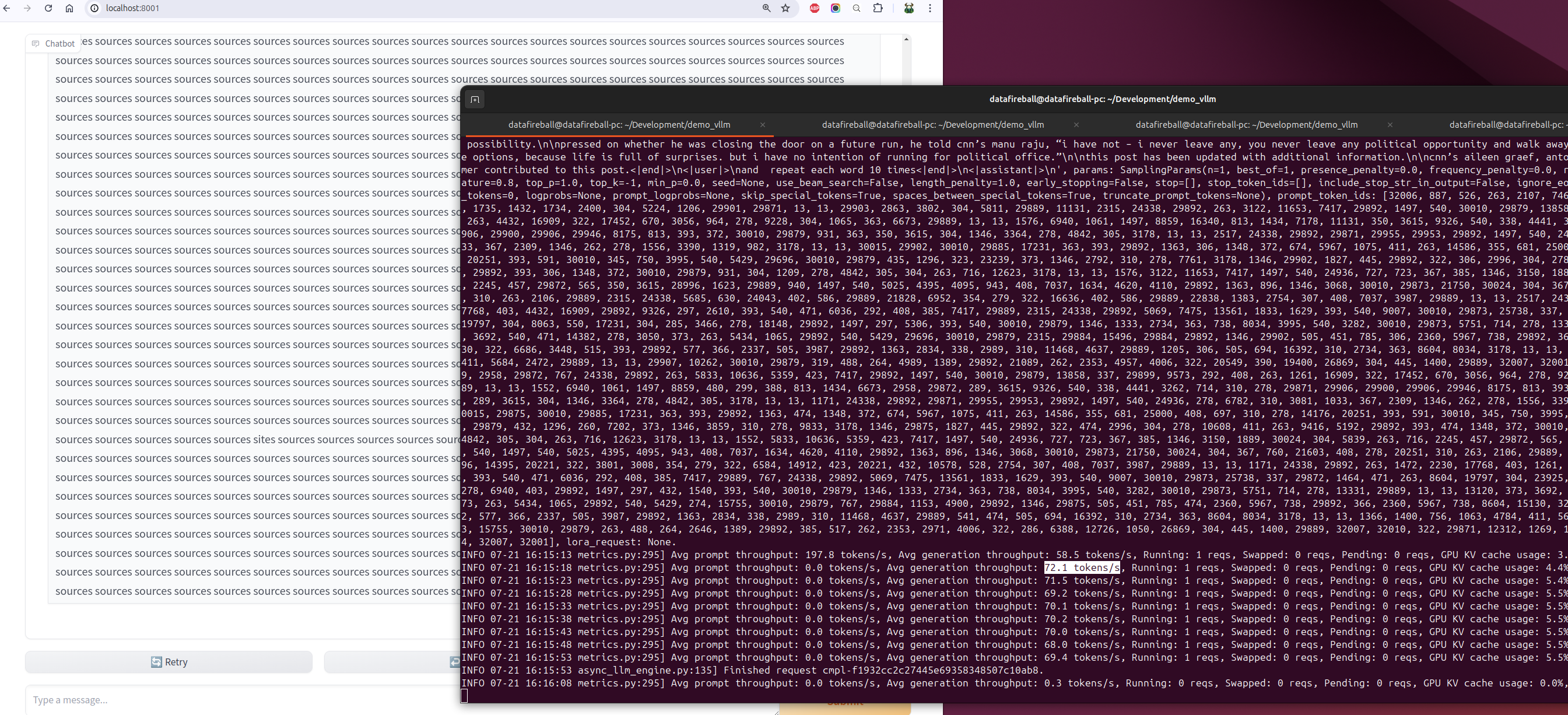
After the model is served, we can interact with the model via API, at this moment, vllm have 3 endpoints implemented, list models (screenshot below), chat completion and create completion endpoints. The vllm API is standardized in a way such that it is a drop in replacement for openai. You can literally take your existing openai code and replace the URL with localhost and your code should just work.
An interesting observation is that the VRAM of 3090 is almost fully occupied, not sure why.
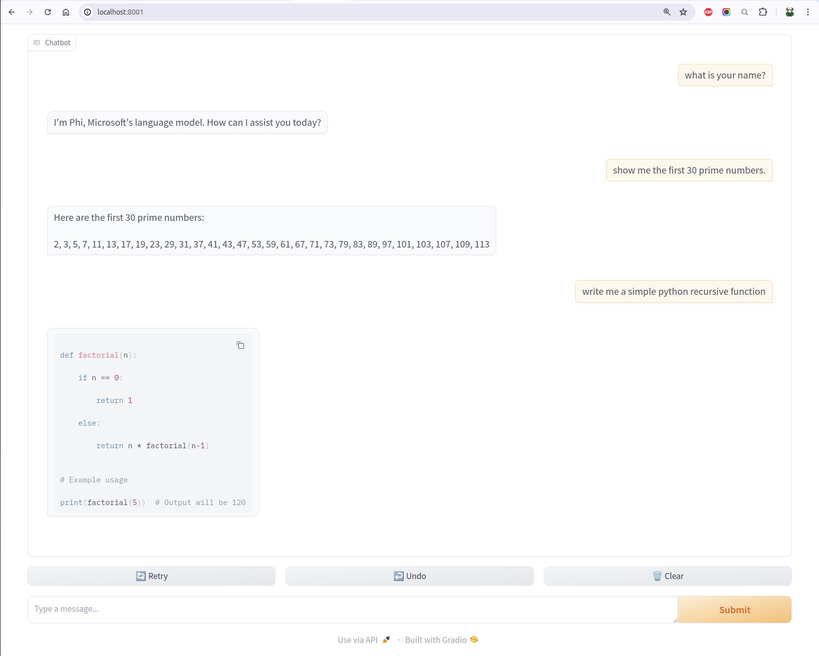
4. Chat UI
vllm comes with many examples. One of the example is to set up a gradio openai chatbot so you can interact with the LLM.
I have heard how even it is to set up model UIs using gradio. By looking into the source code of the UI script, it is so clean and easy, you basically only need to define a predict function by passing it the history and message.
I also tested the throughput by instructing phi to repeat the same word multiple times for a while. During the time of the experimentation, the average generation throughput was about 70 tokens/s.
Just accomplished the short course of pretraining LLM from deeplearning.ai – link
What a good use of a Wednesday night 1 hour’s time, otherwise, I probably will be watching youtube shorts while drinking a beer 🙂
In this tutorial, the instructor Sung(CEO) and Lucy(CSO) from upstage walked through the key steps in training a LLM by using huggingface libraries, mostly importantly, they introduced several techniques like depth upscaling and downsizing to accelerate the pretraining by leveraging weights from existing models but with a different configuration.
The chapter that I personally liked the most is the Model Initialization, this is the step where you customize the configuration and initializes the weights.
For example, here they customized a new model with 16 layers (~308M parameters) and initialized the weights by simply concatenating the first 8 layers from a 12 layers pretrained model and then take the last 8 from the same model. it is like 1,2,3,4, (5,6,7,8,) (5,6,7,8,) 9,10,11,12 and somehow the generate texts have some linguistic coherence instead of completely gibberish.
They claim the depth upscaling and save the training cost by a whopping 70%.
Following the first post of RAG in 5 lines, this post will cover what is happening behind the scene in more detail, what are some of the knobs you can tune so better understand the working internals of llama_index.
llama-index has done such a good job abstracting away the complexities behind the index and query commands. I mentioned that it took me almost 90 seconds to index the 10 articles.
Data Volume
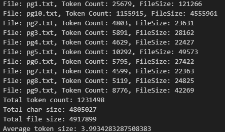
Now let’s look back at how much data that we are working with.
The 10 book occupy about 4.9MB in total in plain text format, by using the cl100k_base BPE, we know they contain in total about 1.2 million tokens. On average, each token takes 4 bytes.
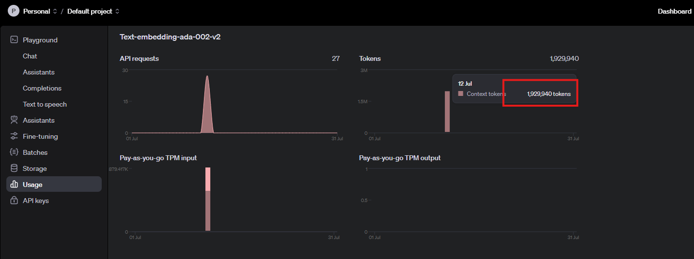
I want to admitthat I had a false start at the beginning. Initially I wanted to index 100 books, then I stopped it after noticing how long the wait was and later changed to 10 books. Now, by noticing that our API usage has 1.9 million tokens in total, that roughly line up with our total number of tokens 1.2 million. (the additional 0.7 million was probably due to my false start).
The theoretical API throughput should be 5M tokens per minute, and our indexing process was about 500K per minute (~10%), this is very slow by default. later on, we can discuss why this happened and how to address it.
Chunk
A key step is RAG is to properly break larger documents into smaller pieces and index them accordingly. In the 5 liner example, there is no place to find the details about how each document is broken down into its own chunks, it is because there are very extensive default settings where the configurations were set there. That means users still have the freedom to customize but if you do not know, there is a default setting for your application.
you can access the default setting by running the following command:
from llama_index.core import Settings
print(Settings)
in the default setting, you can find a lot of useful info like it is using open_ai 3.5turbo as the default LLM and use openai ada002 as the default embedding model. Then you can find they are using the chunk_size of 1024 with a 200 overlap as the sentence splitter.
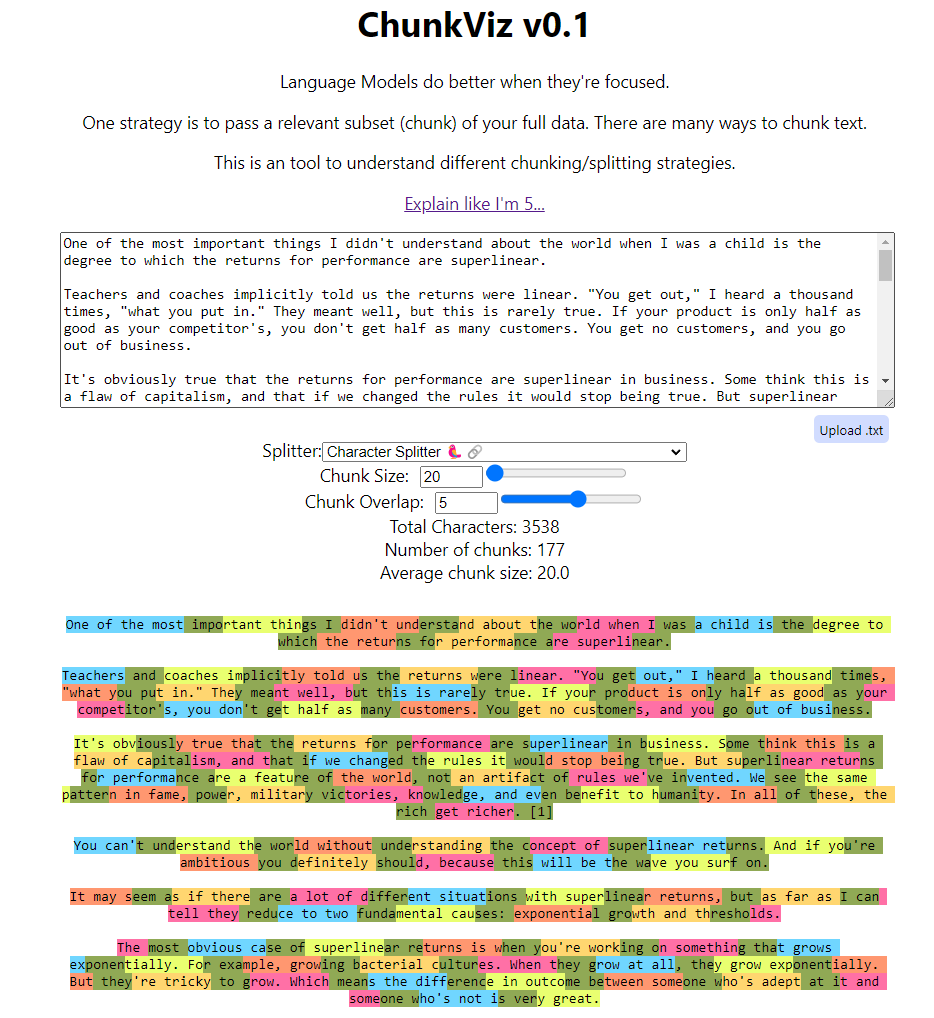
I will not dive too deep into how chunking works, but you should totally check out the ChunkViz from Greg Kamradt.
In the previous section, we know there are about 1.2 million tokens in total. If the chunk size is 1024 with an overlap of 200, we might have ~800 tokens per chunk, which translates to 1.2 million / 800 ~ 1,500 chunks. Now let’s verify whether that was the situation.
>> len(index.docstore.docs)
1583
Document Store
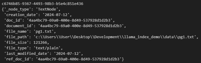
Since now we verified that the raw documents got split into smaller chunks. These smaller documents are now stored in a docstore which is within the index object. as default, the index is using almost a python dictionary which is called SimpleDocumentStore to stores the raw text.
The code below is to iterate through all the docs. Here we print out the first element in the dictionary with its key, its text, number of tokens, and number of characters. Again, we can verify that the token size is within the 1024 chunk size limit and there is on average a 4 to 1 relationship between the number of characters and the number of tokens.
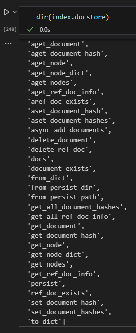
Like any database / store, the document store has many operations mainly around getter/setter, just like the CRUD operations for a database.
Embedding
Embedding is a numerical representation of an entity, in this case, a chunk. based on the default setting, we know they are being batched sent to openai api with a batch size of 100. Given that we have 1,500 chunks, this should translate to 15 requests at most.
Again, it is very likely that we wasted some requests while trying to index 100 docs at the beginning, this verified our hypothesis that the batch indexing is working as expected.
All the embeddings are stored in the vector store.
Vector Store
The vector store is yet another place where all the embeddings are stored, in addition, there are a lot of metadata also stored there representing the underlying document.
for k, v in vs.data.metadata_dict.items():
    print(k)
    pprint.pprint(v)
    break
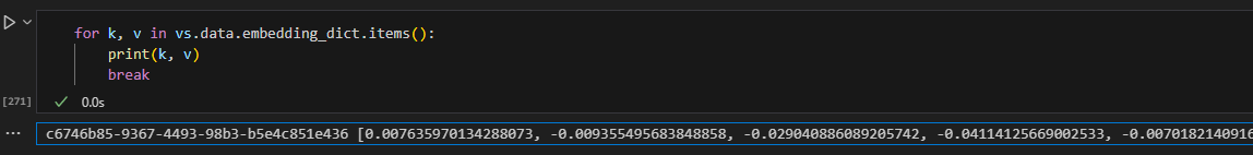
for k, v in vs.data.embedding_dict.items():
    print(k, v)
    break
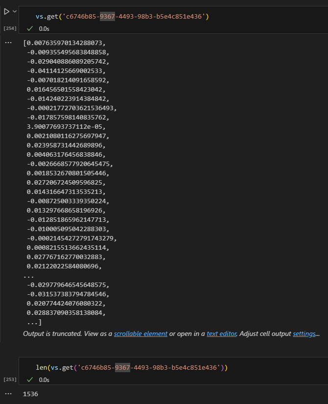
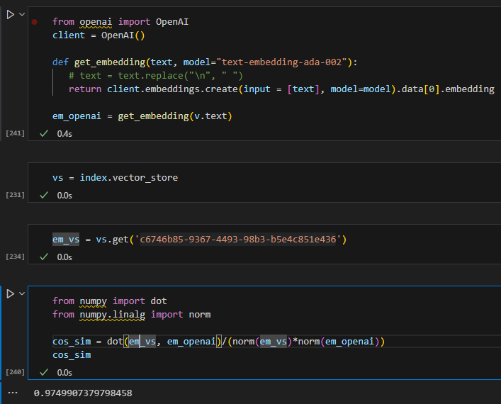
easter egg – not matching embedding
I tried to generate the embedding for a doc myself and compare to its stored embeddings in the vector store, even if they are very similar, I cannot seem to match them 100%. I will not be surprised if there is some pre/post processing somewhere to remove non-printing characters but this is good enough 🙂
Query
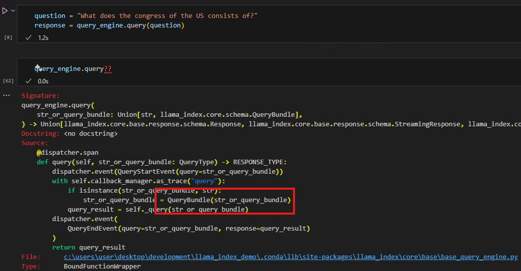
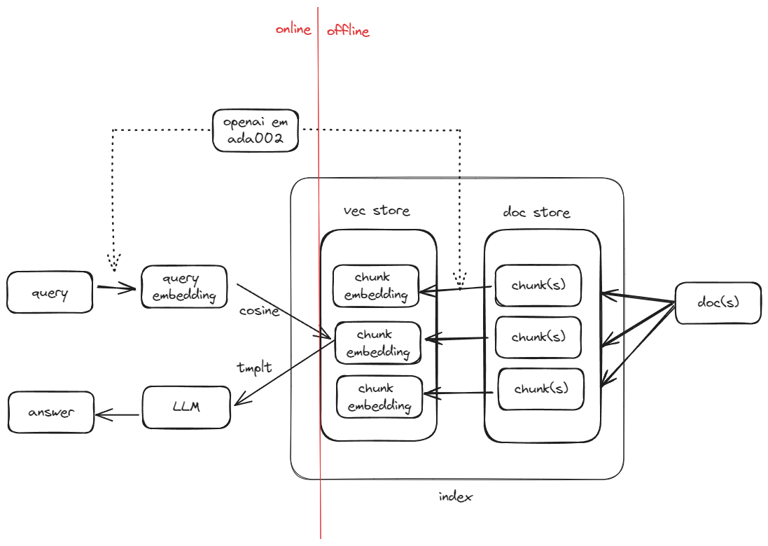
behind the scene of query_engine.query, it converts the query into its embedding and searches it against the vector store to get the best matched record(s). In fact, a simple query_engine will be converted into a retriever which is an synonym in this case.
The code below demonstrated that the query_engine.query will pass in the query as a QueryBundle object.
from llama_index.core.schema import QueryBundle

# Step 1: Generate embeddings for the query
em_query = get_embedding(question)

# Step 2: Create a QueryBundle
query_bundle = QueryBundle(question)

# Step 3: Retrieve nodes using the retriever
retriver = index.as_retriever()
nodes = retriver.retrieve(query_bundle)
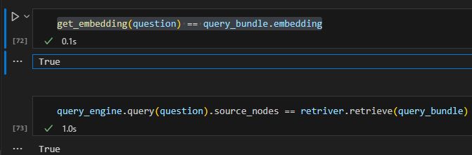
Here we directly calculate embeddings for the query using openai api, and then pass the question to initialize a QueryBundle object that will be used to for retrieval.
Now we can have two observations (at least in this simple 5 liner scenario): 1. query_bundle simply takes the query and embeds it 2. the query_engine.query is running retriever.retrieve behind the scene
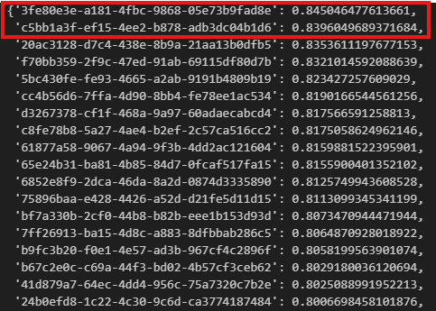
now, let’s try to manually verify the outcome. If we generate the embeddings for the query via openai. Then we can iterate through the vector store and calculate the pairwise cosine similarities, we store the similarities in a dictionary and then we can sort it and highlight the top 2 most similar items.
Based on the outcome, we can verify that the two records 3fe and c5b are the top two results and our similarities match llama-index retrieved too, even their similarity scores match perfectly.
dict_similarity = {}
for k, v in vs.data.embedding_dict.items():
    cos_sim = dot(v, em_query)/(norm(v)*norm(em_query))
    dict_similarity[k] = cos_sim

sorted_dict_similarity = dict(sorted(dict_similarity.items(), key=lambda x: x[1], reverse=True))
sorted_dict_similarity
Synthesis
Now we have located the chunk that is semantically most similar to the query, we still need one more step to further refine in order to provide a concise yet relevant answer. Otherwise, the user is asking “what consistite the US congress”, and we returns a big chunk of text from the constitution for the user to read. This step will need to distill the chunk(s) down to a one or two sentences. In our example, it can even be as short as “house of representative and senate”.
In Llama-index, it is achieved via a component called synthesizer. The retrieved nodes will be served as context, along with the query will be fed directly to a LLM to refine.
l# lama_index.core.prompts.default_prompts.py
DEFAULT_TEXT_QA_PROMPT_TMPL = (
    "Context information is below.\n"
    "---------------------\n"
    "{context_str}\n"
    "---------------------\n"
    "Given the context information and not prior knowledge, "
    "answer the query.\n"
    "Query: {query_str}\n"
    "Answer: "
)
RAG is taking over the world as an augmentation or even replacement to traditional search. It has claims like context augmented leveraging LLM. Through new techniques like LLM and vector search, it offers a new way to offer better quality responses to users. This article is meant to demonstrate how RAG works in the bare minimal example.
Llama-index is one of the the most popular libraries these days for building a rag and its has its famous 5-line starter:
from llama_index.core import VectorStoreIndex, SimpleDirectoryReader

documents = SimpleDirectoryReader("data").load_data()
index = VectorStoreIndex.from_documents(documents)
query_engine = index.as_query_engine()
response = query_engine.query("Some question about the data should go here")
print(response)
Before running the code, we need few preparation steps:
OpenAI Key
To leverage the LLM part, the easiest way is to just call openai api, once you create a key and place it under .env file, you can load into the environment variable as a best practice.
import os
import dotenv
dotenv.load_dotenv()
print(os.environ['OPENAI_API_KEY'])
Books Data
We need some toy data to work with, Gutenberg books is a good place to get some free books. The code below will download the first 10 books from gutenberg project by manipulating the url. The books will be stored in a local directory – data. (precreate it if it does not exist yet)
number_of_books = 10
for i in range(1, number_of_books+1):
    url = f'https://www.gutenberg.org/cache/epub/{i}/pg{i}.txt'
    response = requests.get(url)
    if response.status_code == 200:
        with open(f'./data/pg{i}.txt', 'w') as f:
            f.write(response.text)
    else:
        print(f'Failed to download {url}')
Load the Data and Index
docs = SimpleDirectoryReader('data').load_data()
index = VectorStoreIndex.from_documents(docs)
query_engine = index.as_query_engine()
The three lines above is all you need to load the data, create an index and set the index to be used as query engine. The index initialization took me a while (1minute and 30 seconds) to index the 10 books. So let’s put it into action.
Query
The first few books that we downloaded happen to literatures at the establishment of the US, which also includes the US consistitution, so lets try to ask a question and see how it works.
>> response = query_engine.query("what does the congress of the US consists of?")
>> response

Response(response='The Congress of the United States consists of a Senate and House of Representatives.', source_nodes=
voila, we got the answer that we need!
In the next post, we will dive into each of the building blocks and understand what is happening behind the scene.
For a long period of time, developers use RESTful APIs to pull data from services and build website on top of it. A disadvantage of REST is users tend to spend a lot of time playing with the query parameters and parsing the outputs because frontend is constrained by the backend, sometimes only need a single data point from a heavy requests that is quite wasteful. GraphQL is a way to enable frontend developers to selectively prescribe what to pull and backend will only focus on what to feed, making the communication super versatile, and efficient after all. GraphQL is more about about the “QL” – query language and less about the “Graph”. During my first encounter with GraphQL, I found a great resemblance of GraphQL with SQL, you define your schema and users “query it”.
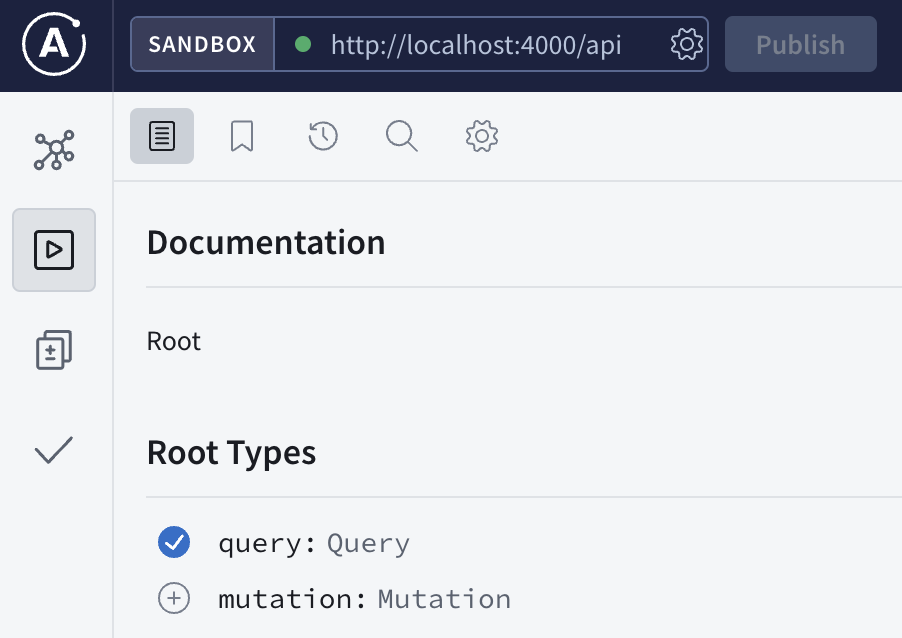
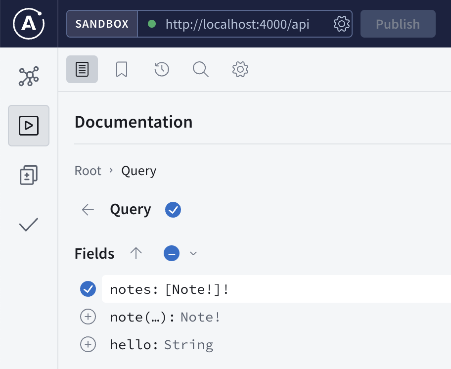
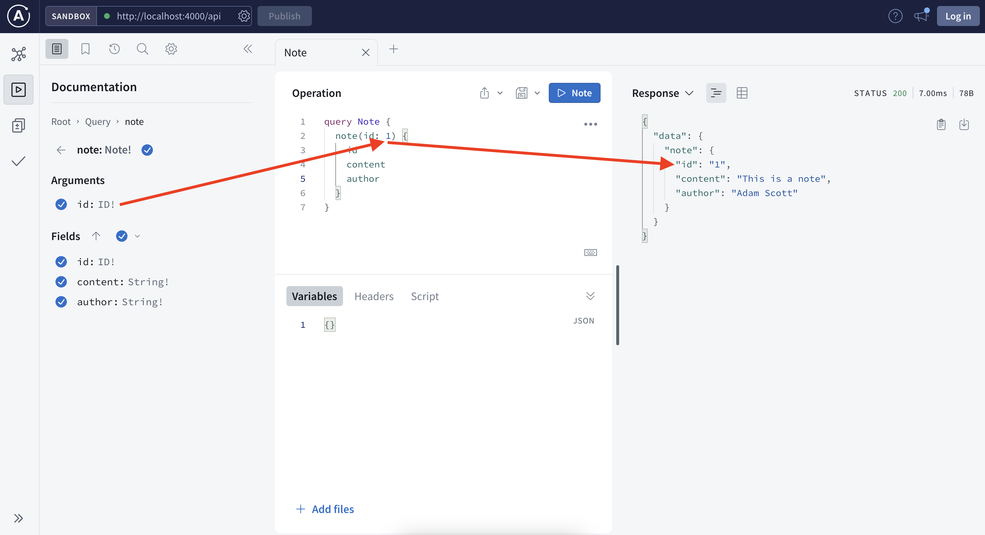
Just like a SQL table, one needs to know the schema of the data first before using it. Above is a screenshot of the GraphQL schema visualized in apollo explorer.
We know there are 3 fields (columns) that we can query, the hello field will return helloworld for testing purpose, notes to return a list of all the notes and note to return a specific note.
In this simple example, there are 3 fields available to query, and each field can have 3 attributes that you can customize. Depending on the use cases, some users may only need the content, some may only need authors, some may need all fields, if you take all the combinations of different user cases into account, it is very hard to expect all the users cases. Instead, GraphQL defines the schema with all the ingredients available, and the users just need to query what they need.
The explorer is very helpful to interact, by nature, it is just a typical HTTP request with the graph query in a json format stored in the payload. See below, you can also choose between inline variable or extract variable and both works.
How to Build it
Define Schema
gql“ in Javascript represents a tagged template literals, it parses the GraphQL schema language the typeDefs object will need to be passed to the apollo server during initialization.
Define Resolver
The schema defines the “what”, and the resolver takes care of the “how”. In this simple example, the Query block defines how the three query works.
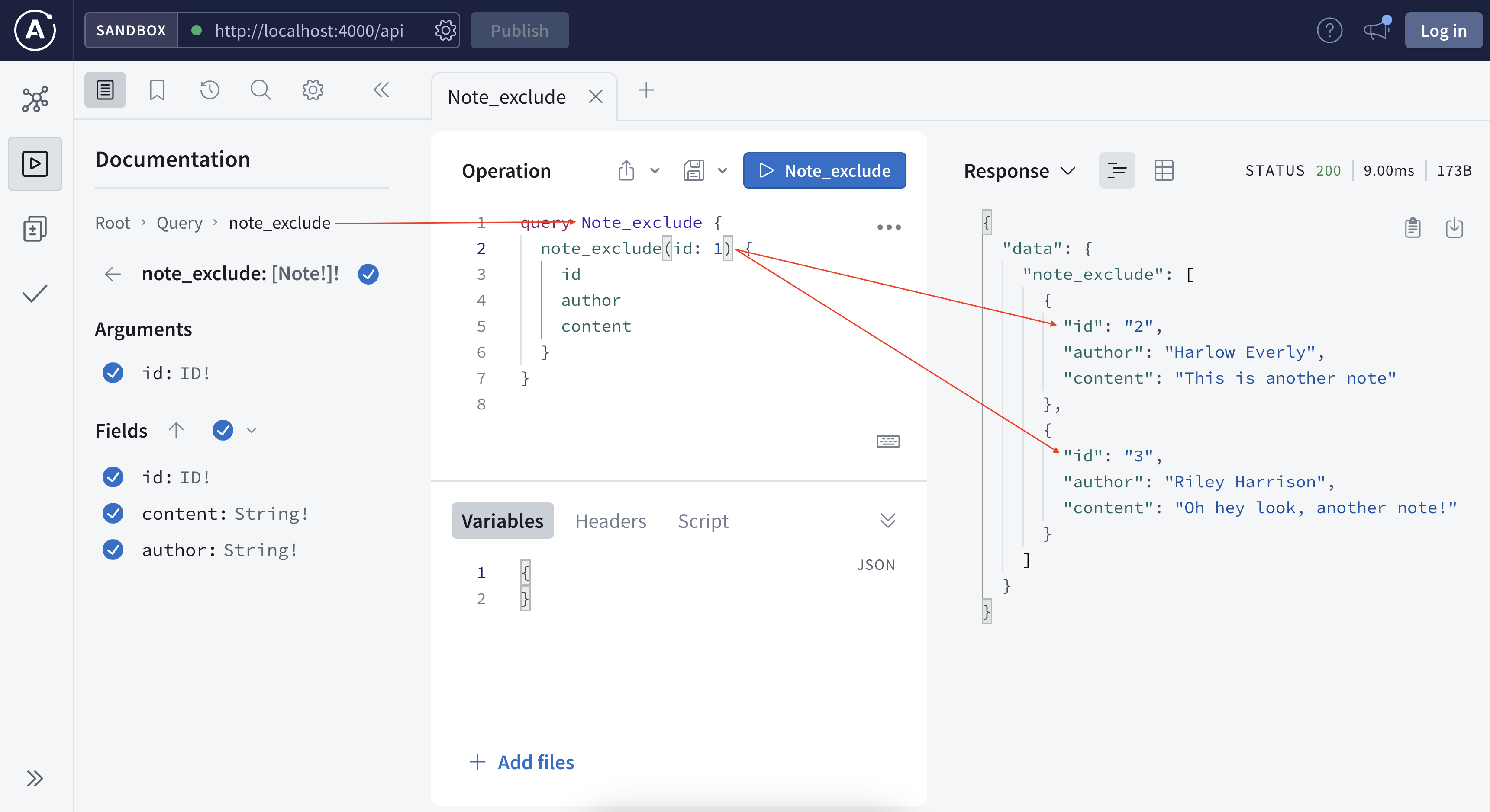
Try it Yourself
Now we saw how the schema and resolver work together. Let’s try to add a new field so it returns all the notes but the one specified by the user (this may apply to feed new unread articles).
Where is the Graph
We just covered the query language part, now let’s think about where is the graph. There is a great article by Bogdan discussing about the graph part of GraphQL.
You can also visualize any graphql using a tool called graphvoyager.
More Questions
if graphql query ended up being a DAG, given different steps might take different time, is this also an optimization problem as there may be a goal of minimizing the total execution time or maximizing the total throughput, aka, the job scheduling problem.
Luna Dong Podcast – Building the Knowledge Graph at Amazon with Luna Dong Three key features of Knowledge Graph: 1. structured data (entities and relationships) 2. canonicalization/rich/clean 3. data are connected In Amazon, there exists separation of digital product from retail products because the former tend to have better and more well structured metadata, the retail products tend to require to extract digital data from various kinds of real life data for example (images, raw texts, …)
“is-a” relationship, “event” information, use the “seed knowledge” to automate the building of train data. The more you know, the faster you learn.
Knowledge Extraction: from web, product description (text, …) web tables, product data is collected from text and images
Data Integration: “is_a_director_of” is the same as “director” relationship, database and NLP community, we put things together to decide whether two things are wrong by looking into inconsistency (color, product flavor, data sources). Data fusion is to decide which version is right – is this person’s birthday on Feb 28th or Mar 28th? Through this process, you can learn embeddings that can be used for downstream tasks like search, recommendation, Q&A and many others.
Human in the loop is important because we need high quality data, it is important to seed the training data, annotate the data and calibrate and analyze the overall performance, and it is also important to address the last mile failure if we want to be 99% accurate.
The most inspiring moment from Luna is from Amazon’s fulfillment center, to combine machine power and human power.
Data acquisition: the product manufacturer’s website contains a lot of information, start with general crawling and sometimes do targeted crawling. It is not a binary, it is a mixture.
Embedding: conditional embedding. spicy is a valid flavor, spicy is unlikely to be part of an ice cream flavor, capture these constraints in an implicit way, these spicy flavor in general can be covered in certain types of products.
Triple – subject-predicate-object, look at all the triples together, and clean the embeddings from that way, the embeddings can propagate in the graph. Some products have the flavor spicy. Graph neural network is one of the most effective way to solve the problem.
The knowledge graph is a production system, the knowledge is generated from a lot of products – there are three major applications – search (intent), recommendation (similarities but still some difference), display of information (structured information and structured knowledge, better comparison table).
Luna said most knowledge graphs are built and owned by large corporations, she wishes there are tools for smaller business. She said there are three levels, first being the database and tooling storing knowledge graphs, the second being the techniques to entity and relationship extraction.
Open knowledge is an effort to connect and hook up different data sources.