Mongodb – Move Collection to Another Mongo Server File Size Analysis

You can check the stats of a mongodb collection by using the command below:

db.<collection>.stats()

> db.seCrossReferences.stats()
{
“ns” : “result.<collection>”,
“count” : 256292,
“size” : 3049450896,  # which is about 2.8GB
“avgObjSize” : 11898.346011580541,
“storageSize” : 4109500416,
“numExtents” : 18,
“nindexes” : 1,
“lastExtentSize” : 1071394816,
“paddingFactor” : 1,
“systemFlags” : 1,
“userFlags” : 0,
“totalIndexSize” : 8323168,
“indexSizes” : {
“_id_” : 8323168
},
“ok” : 1
}

Then you can export/dump the data using mongoexport or mongodump, the syntax for mongodump is as follows, it will dump the binary data out of mongo and save to a directory:

################### MONGODUMP ####################################

mongodump –db <dbname> –collection <collectionname> –out <outputpath/name>

It turns out that the size of the dumped folder is about the same size as what is showed in the db.<collection>.stats(), which makes sense because the dumped result is in binary format, result.bson.

Then you can use gzip to make it into a tar ball where the file size is only 177MB, which is less than 7% of the original file.

You can also dump the file to standard output and gzip on the go in one liner:

mongodump –db <dbname> –collection <collectionname> –out – | gzip -9 > <outputfilename>.gz

it took 6 minutes in total to dump and gzip the file, -9 flag make sure it is the best compression rate, but after all, the file size is 171 MB which is almost the same.

################### MONGOEXPORT ####################################

mongoexport will export the mongodb data to a human readable file JSON/CSV. The command syntax is similar and lets take a look:

mongoexport –db <dbname> –collection <collectionname> –out <outputfilename>.json

The exported json format file is 2.9 GB in this case and it took about the 7 minutes also.

mongoexport –db result –collection seCrossReferences | gzip > seCrossReferences.json.gz

This takes about 10 minutes but… the exported zipped file is 144MB…

In conclusion, I think maybe mongoexport + zip is a better solution, because:

1. its output is json/csv which could be used for something else except for moving database.

2. the output has a smaller size

############# IMPORT DATA #######################################
mongoexport + mongoimport
mongoimport –db –collection –file .json –type json

mongodump + mongorestore
http://docs.mongodb.org/manual/reference/program/mongorestore/

Scrum – Agile Software Development

Scrum is an iterative and incremental agile software developmentframework for managing software projects and product or application development. It defines “a flexible, holistic product development strategy where a development team works as a unit to reach a common goal”. It challenges assumptions of the “traditional, sequential approach” to product development. Scrum enables teams to self-organize by encouraging physical co-location or close online collaboration of all team members and daily face to face communication among all team members and disciplines in the project.

A key principle of Scrum is its recognition that during a project the customers can change their minds about what they want and need (often called requirements churn), and that unpredicted challenges cannot be easily addressed in a traditional predictive or planned manner. As such, Scrum adopts an empirical approach—accepting that the problem cannot be fully understood or defined, focusing instead on maximizing the team’s ability to deliver quickly and respond to emerging requirements.

Reference: http://en.wikipedia.org/wiki/Scrum_(software_development)

Nutch Hadoop

Nutch Hadoop Tutorial – This is a tutorial that shows you how to set up Apache Nutch on a running hadoop cluster and won’t dive into the architect detail too much, which is a perfect tutorial for me. 

A few assumptions before following this tutorial:

1. root 2. ssh 3. cluster 4. maillist for Q&A 5. Java programming background

Hadoop Cluster Setup:

Download Hadoop and Nutch:

Setup the Deployment Architecture

Deploy Nutch to a Single Machine

Deploy Nutch to multiple Machines

Performing a Crawl

Testing the Crawl 

Performing a Search


MNIST databse – the Have-To for Image Recognition

I randomly came across a post from Kaggle, which is actually part of a tutorial competition showing people how to get started with machine learning.

More information about the famous MNIST dataset, which is used in this competition, could be found here. I remembered that Andrew Ng’s online class has demonstrated how to do image recognition, using different types of algorithms. However, while I was taking his class from Coursera, the software the class used was Octave. I am mostly using R and I want to give it a try with R.

After I downloaded those MNIST dataset files, again, I realized it is not that easy as I expected. All the files are in binary format and I have never dealt with binary files in R. After a quick good, I know there is a file named after me :), “readBin”. And fortunately, I found a paragraph of R code in git written by brendano, which works out of box.

However, 知其然知其所以然(we should know the hows and also the whys). Here is a very useful post from IDRE – Institution of Digital Research and Education from UCLA.

If you think binary data set is  faraway from your life, you are wrong. The `save` command in R, actually store the data in binary format. “Saved R objects are binary files, even those saved with ascii = TRUE, so ensure that they are transferred without conversion of end of line markers and of 8-bit characters. The lines are delimited by LF on all platforms.”

R – aov Plus TukeyHSD to quickly identify difference between categories

Say you have a column which contains categorical variables / factors. Then How can we quickly and confidently identify the differences between different categories?

A very commonly used dataset ‘mpg’ from the package ‘ggplot2’ contains some categorical variables that could easily get started. There is a column in mpg called ‘cty’ which is the miles per gallon for a car while driving in city. And also another column ‘manufacturer’ which contain categorical variable the different manufacturers.

library(ggplot2)
data(mpg)
bymedian = with(mpg, reorder(manufacturer, -cty, median))
boxplot(cty ~ bymedian, data = mpg, varwidth = TRUE)

result = aov(formula = mpg$cty ~ as.factor(mpg$manufacturer))
TukeyHSD(result)

aovmpgmanufacturer

mpgboxplotmanufacturer

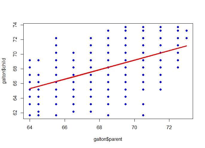
Francis Galton: relation between the heights of children and the height of their parents.

Background Story:

Sir Francis Galton, who is the cousin of Charles Darwin was an English Victoria polymath, eugenicist and statistician. He proved the linear combination of normal distribution is still normal distribution and he is also,the inventor of the triangle device – quincunx. Here, we will talk about the research that he has implemented long time ago(1885).

library(UsingR)
data(galton)
par(mfrow=c(1,1))
plot(galton$parent, galton$child, pch=19, col=”blue”)
m <- lm(galton$child ~ galton$parent)
lines(galton$parent, m$fitted, col=”red”, lwd=3)

Image

R – Interesting Density Plot

I always use histogram command to look at the distribution of a uni-variable data. And to distinguish the difference of distribution of a subgroup from the whole, I usually do two or more plots with the same scale.

data(mtcars)
par(mfrow=c(4,1))
hist(mtcars$mpg, breaks=20, col=8, xlim=c(10, 40), main=’total’)
hist(mtcars$mpg[mtcars$cyl==4], breaks=20, col=3, xlim=c(10, 40), main=’V4′)
hist(mtcars$mpg[mtcars$cyl==6], breaks=20, col=4, xlim=c(10, 40), main=’V6′)
hist(mtcars$mpg[mtcars$cyl==8], breaks=20, col=5, xlim=c(10, 40), main=’V8′)

Image

You can clearly read the information that the more cylinders you have in your car, the more gas it will take in general, of course, a lower MPG (Miles Per Gallon).

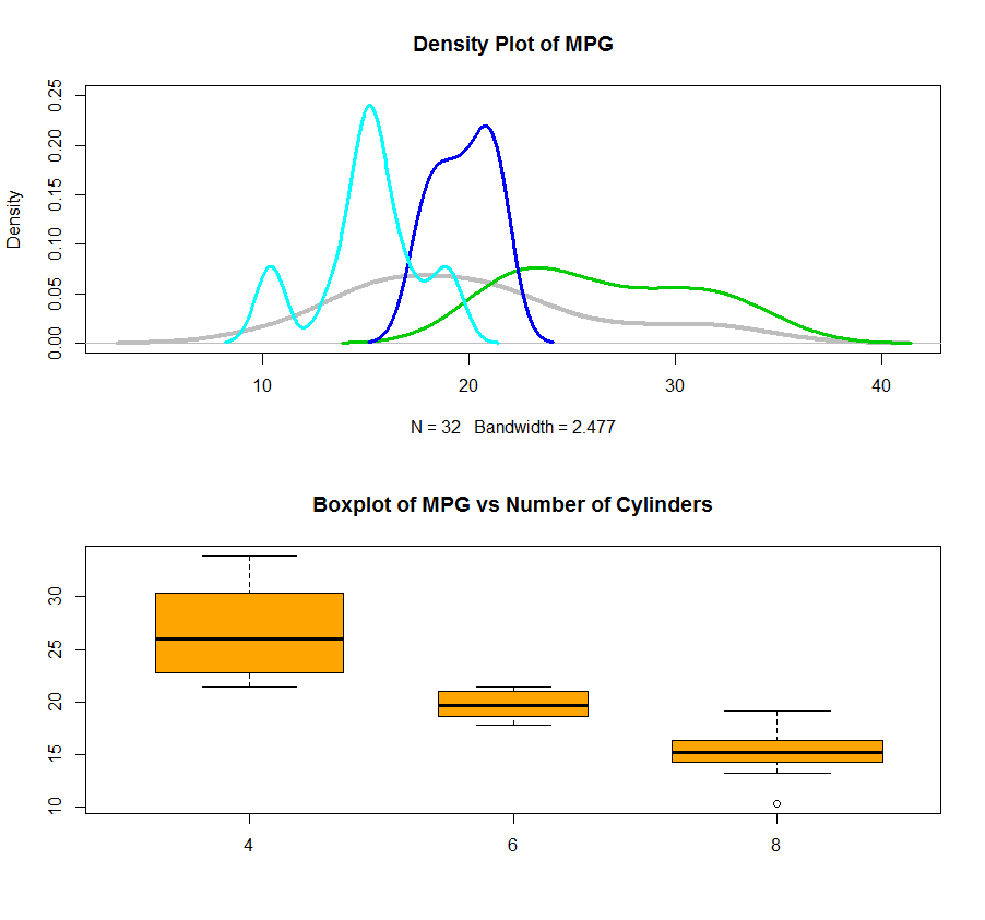
Also, you can use the density plot to see the distribution of data for each cylinder and plot them all together in one plot. I also attached a boxplot using factor which give a better picture of what is going on. By the way, the varwidth=TRUE will set the width of the box as the number of records in that box. In this case, you will see we have almost same amount of records inside each category.

dens = density(mtcars$mpg)
dens.4 = density(mtcars$mpg[mtcars$cyl==4])
dens.6 = density(mtcars$mpg[mtcars$cyl==6])
dens.8 = density(mtcars$mpg[mtcars$cyl==8])
par(mfrow=c(2,1))
plot(dens, lwd=4, col=8, ylim=c(0, 0.25), main=”Density Plot of MPG”)
lines(dens.4, lwd=3, col=3)
lines(dens.6, lwd=3, col=4)
lines(dens.8, lwd=3, col=5)
boxplot(mtcars$mpg ~ as.factor(mtcars$cyl), varwidth=TRUE, col=’orange’, main=”Boxplot of MPG vs Number of Cylinders”)

densityboxplotmtcarsmpg