A key step in preprocessing prior to training a model is to properly split the dataset into training, validation and test datasets. In traditional machine learning, the dataset is usually a dataframe/table like where each column represents a feature and each row represent a record. Due to the simplicity in that structure, the split can be as easy as rolling a dice to determine which records goes to which bucket, you can find the source code for sklearn model_selection.train_test_split. However, the data structure for a graph dataset is different, it contains nodes and edges, in addition, it contains attributes and labels for nodes and edges. For a heterogenous graph, it can be more complex with different types of nodes and edges. Given those challenges, torch_geometric is “battery-included” with a function train_test_split_edges for edge prediction. In the latest documentation, train_test_split_edges is deprecated and is replaced by  torch_geometric.transforms.RandomLinkSplit, in this post, we will only cover train_test_split_edges due to its simple implementation. Before we dive into the specifics, let’s first take a look at popular ways of splitting data and its best practices.

Cora

Cora dataset is a popular graph dataset. it describes the citation relationship between scientific publications, there exists 5429 links and 2708 entities and 7 classes representing a domain the publication belong to.

GCN (graph convolutional network) has been considered a bedrock for graph machine learning, in the paper where GCN is being considered invented – semi-supervised classification with graph convolutions networks. The author Kipf and Welling used the cora dataset.

However, instead of using all the links for training, they only picked 20 samples per class, given there are only 7 domains, the training dataset is only 140 records which is merely 2% of the whole dataset. And they used 500 (9%) for validation and 1000 (18%) for testing. The volume of training data can even be considered disproportional comparing to most supervised learning where very majority of the data goes to training if not all.

This is a common practice in semi-supervised learning on graphs, where the goal is often to learn from a small amount of labeled data (the training nodes) and to generalize this to the unlabeled data (the test and unused nodes).

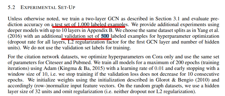
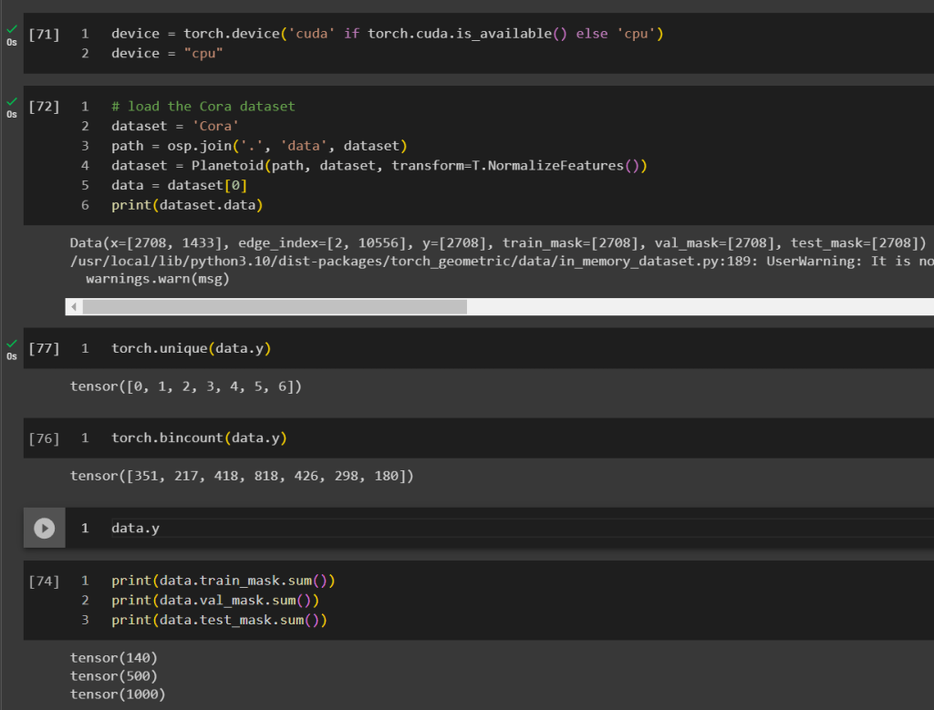
This may not be a perfect example as it is a node classification problem but it is a good conceptual example demonstrating it is critical to preprocess the dataset by splitting them right.

Next, let’s take a look at for a link prediction task, how to split the links into train, validation and test.

train_test_split_edges

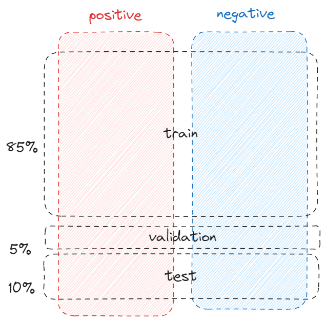
By default, train_test_split_edges splits the dataset into 3 categories, 5% goes validation, 10% goes to test and the rest 85%=1-5%-10% goes to training. However, the link prediction is a binary classification by nature, so we need to have positive cases (relationship exists between two nodes) and negative cases (relationship doesn’t exist between two nodes).

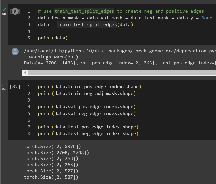
If the dataset is already loaded into torch_geometric, you can just run train_test_split_edges on the data object.

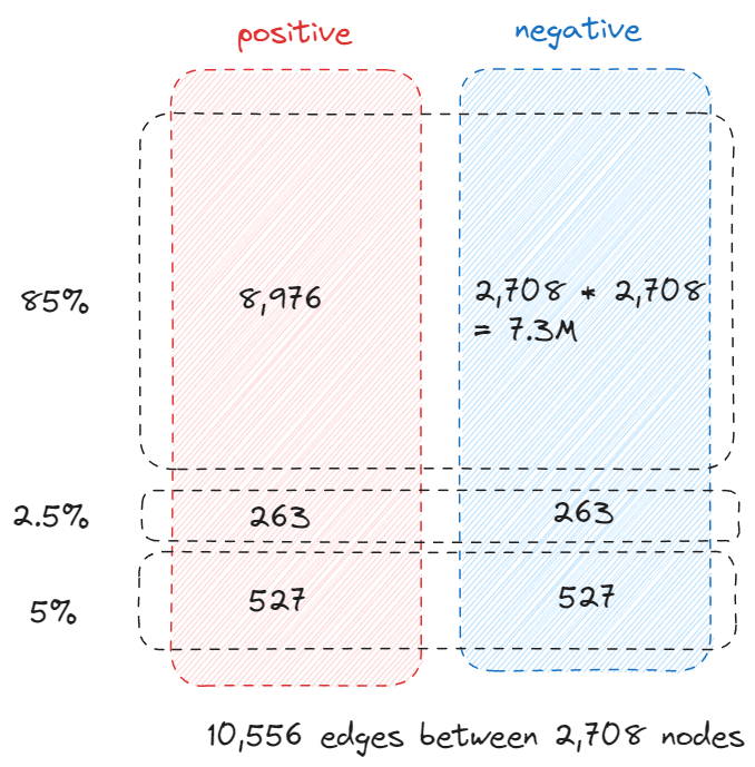
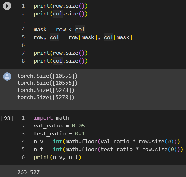
An interesting observation is that the validation and test edges is 2.5% and 5% of the total edges instead of the 5% and 10% we previously mentioned, soon you will know why.

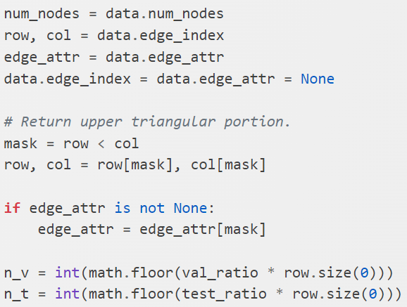
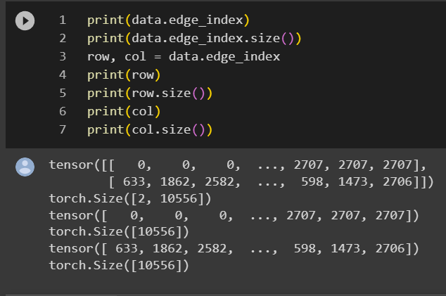
row stores all the source node of all the links and col stores all the destination nodes. They have the same size as the number of links which is 10,556. Consider there are 2,708 nodes, technically the adjacency matrix should have the size of 7.3M, 10,556 is only 0.14% of 7.3 million so storing the links in this way (COO – coordinate format) is very efficient.

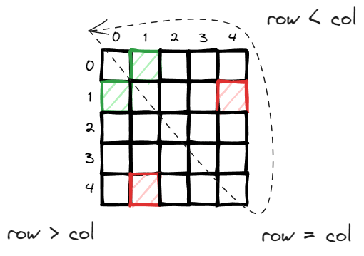
in an undirected graph, you can consider either direction and it is efficient to consider only half of the adjacency matrix, in this case, the top right upper triangle (diagonal is self directed link which can be ignored).

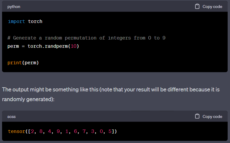
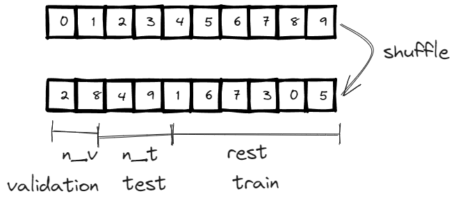
Below is the implementation, the concept is very straightforward and in addition to the index for train/validation/test, if the edge attribute is available, it is also stored in the corresponding edge_attribute.

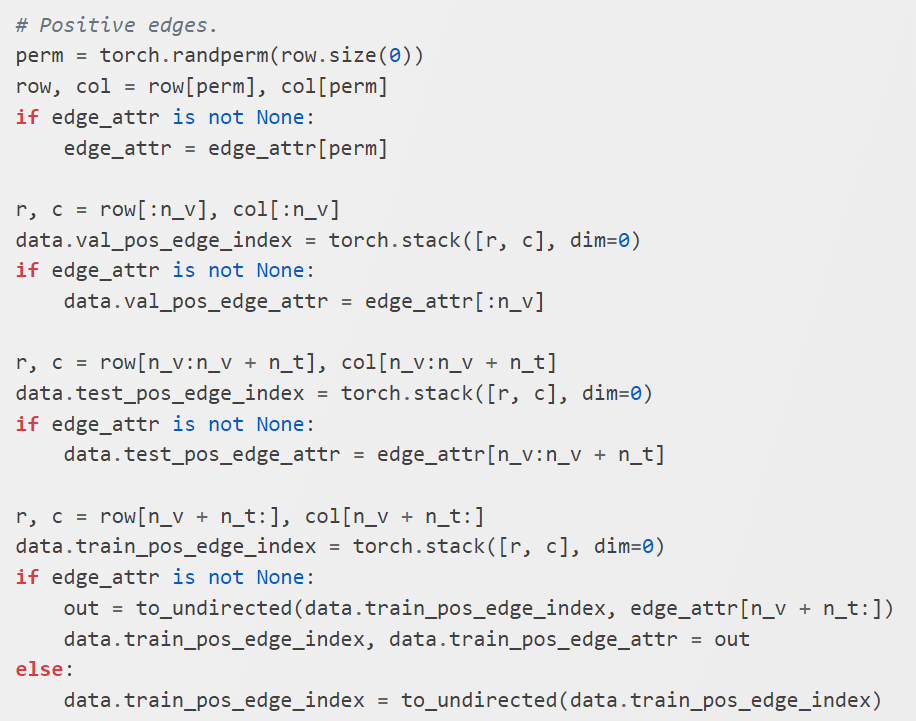
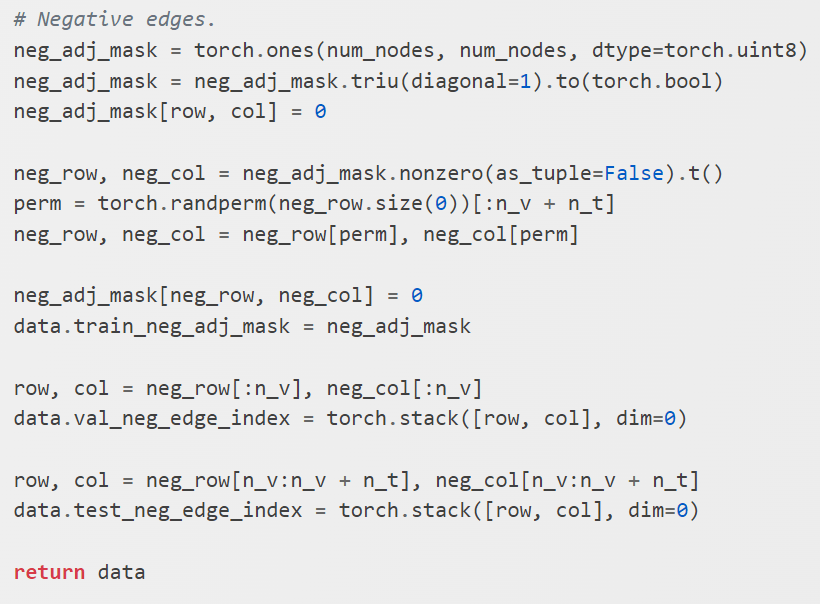
The negative samples are handled differently due to the fact that what is not there implicitly considered negative samples, and it is usually 100x bigger if not 1000x than the positives samples.

First, they construct a full adjacency matrix where each cell has the value of one. And then mark all the existing edges as 0 and find all the remaining ones as negative samples. Then it extracts all the indices using tensor.nonzero.

From the negative samples, it first extracts n_v + n_t many samples as negative samples which corresponds to the same number of samples for positive validation set and test set. After that, it update the neg_adj_mask to exclude those allocated samples.

This is the beauty of this technique. There are significant amount of negative training samples. Instead of storing them like positive samples or negative validation set and test set, we decide to keep track of the huge population by using the neg_adj_mask instead of COO format, this way.