Customize the Python in PySpark

In the data booming age, there is an unprecedented amount of demand for data processing, especially “big data scale” processing, something that you just know it won’t work on your laptop. A few common cases like parsing large amounts of HTML pages, preprocess millions of photos and many others. There are tools readily available if your data is fairly structured, like Hive, Impala but there are just those cases, which you need a bit more flexibility other than plain SQL. In this blog post, we will use one of the most popular frameworks Apache Spark, and share how to ship out your own Python environment without worrying at all about the Python dependency issues.

In most of the vanilla big data environment, HDFS is the still a common technology where data is stored. In Cloudera/Hortonworks distribution and cloud provider solutions like AWS EMR, they mostly YARN or Hadoop Next Gen. Even for an environment where Spark is installed, there are many users run Spark on top of YARN like this. As Python is the most commonly use language, Pyspark sounds like the best option.

Managing Python environment on your own laptop is already fun, managing multiple versions, multiple copies on a cluster that likely be shared with other users could be a disaster. If not otherwise configured, pySpark will use the default Python installed on each node. And your system admin certainly won’t let you mess with the server Python interpreter at all. So your cluster admin and you might come to a middle ground which a new Python, say Anaconda Python, can be installed on all the nodes using a network shared file system which you have more flexibility, as any installation can be mirrored to other nodes and the consistency is ensured. However, only after a few days that you noticed your colleagues accidentally “broke” the environment by upgrading certain libraries without you knowing, and now, you have to police that Python environment. After all, this comes to the question of how each user can customize their own Python environment and make sure it runs on the cluster. The answer to Python environment management is certainly Anaconda, and the answer to distributed shipment will be YARN archives argument.

The idea is that for any project, feel free to create your own conda environment and do the development within that environment, so in the end, you will use the Python at your own choice and a clean environment with all the necessary libraries only installed for this project. Like a uber jar idea of Java. Everything python related in one box. Then, we will submit our pyspark job first by shipping that environment to all the executors where the workload will be distributed, but then second, configuring each executor will use the Python that we shipped. All the resource management, fan out and pull back will be handled by Spark and YARN. So three steps in total, first being a conda environment, second being a Pyspark driver and last is the code submition.

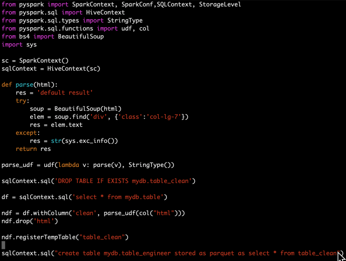
In the following section, I will share how to distribute the HTML parsing in a Cloudera environment as an example, every single step is also available on Github in case you want to follow along.

Conda

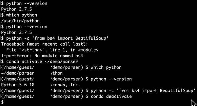
If you are not already familiar with Conda, it is only one of the tools that many Python users live and breathe on a day to day basis.  You can learn more about Anaconda from here.
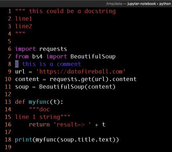
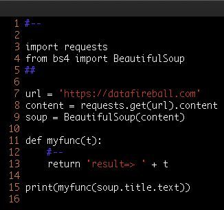
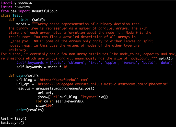
Screen Shot 2020-04-11 at 2.53.43 PM

Driver.py

Screen Shot 2020-04-11 at 2.41.10 PM

Run.sh

Screen Shot 2020-04-11 at 2.37.55 PM


Reference:

[1] https://docs.cloudera.com/documentation/enterprise/5-14-x/topics/spark_python.html

[2] https://blog.cloudera.com/making-python-on-apache-hadoop-easier-with-anaconda-and-cdh/


ssh tunneling via port 22.

Recently I got access to a server that somehow all the ports got blocked except for SSH, instead of waiting for a few weeks until the IT freeze and ports got opened up, I found that you can access the other ports via a technique called SSH tunneling if you have admin rights on the remote host.

ssh -L 9191:localhost:9191 -L 8080:localhost:8080 -L 8088:localhost:8088 user@host

This will ssh into the remote host and keep those three ports mapped from local client to remote host. However, this is fragile as if your ssh is broken, all the ports will be broken, and if your terminal is idle with a broken pipe, your tunnel is also break. There are other flags like run in background as daemon but if you chose that route, make sure you kill the ssh process when done, otherwise, you will never get back to your own 9191 🙂

Screen Shot 2020-04-05 at 11.21.20 PM

Now you can access the port in your client browser just like below.

Screen Shot 2020-04-05 at 11.21.57 PM

Converting Alpha only images to RGB

There are plenty of images data out there that are of the format RGBA (Red Green Blue and Alpha), in which Alpha represents the transparency. By leaving RGB all empty and Alpha to store the information of the shape, the image itself is like a layer that you can add on top of any other photos that sort of “float around”, just like lots of icons out there. However, this type of photos aren’t necessarily friendly or ready to be directly fed into many of the machine learning frameworks which usually work with RGB or greyscale directly. This is a post to document what I did to convert some of this kind of alpha only images into RGB image.

First, there are plenty of libraries out there process images. I am merely sharing some of the work that I did without necessarily comparing the performance of different approaches. The libraries that I will cover in this post is imageio and Pillow. I have read htat imageio is supposed to be your first choice as it is well maintained while Pillow isn’t anymore. However, I found that imageio is very easy to use but its functionality is limited and not as diverse as Pillow. Imageio, as the name indicates, deals with read and write of images, while Pillow has more functionalities of dealing with images itself like channels, data manipulation, etc.

My very first try was to convert RGBA into a matrix that has (200, 200, 4) which my image already has the square size of 200×200. And then drop the last column which is alpha and then populate the RGB channel using the value of alpha channel. In that case, our RGB will be equally populated and our photo should look black and white.

Screen Shot 2020-04-05 at 10.59.27 PM

The code is simple, m is PIL.Image.imread returned object. I first resize it to be 256*256, which is more ML friendly. And then convert it into an array, data which has the shape of 40000, 4. After assigning RGB and dropping A, we call the reshape to turn it back into 256*256*4 and reconstruct the image “fromarray”. Here astype(np.unit8) caught me offguard a bit and there maybe one of the reasons that Pillow is not perfect due to the lack of maintenance. And the invert in the end will invert the color (black to white and white to black) so it has the background that I like.

The code is easy to understand but when I execute it, it was slow, I did not run any benchmark but it was noticeable slow comparing with some other preprocessing that I ran before.

In the end, I realize that there is already a built in function called getchannel so you can get a specific channel without dealing with arrays directly.

Screen Shot 2020-04-05 at 11.04.11 PM

The convert_rgb_fast does the same thing as the function above but execute much faster, likely because I was doing lots of matrix assignment and index slicing which is not very efficient I guess.

Also, by using getchannel, you can easily convert it to have only one channel that is basically greyscale. All the channels don’t have name and RGBA is just convention, if you only have one channel, all the tools out there will assume it is greyscale.

Screen Shot 2020-04-05 at 11.07.47 PM

Image preprocessing is likely as important as training the model itself, the easy part of image processing is that it can be easily distributed using frameworks like mapreduce, spark and others. Using Python is probably the easiest way for model data professionals and we will find an opportunity in the future to demonstrate how to speedup the data cleaning.

stylegan2 – using docker image to set up environment

First, here is the proof that I got stylegan2 (using pre-trained model) working 🙂

Screen Shot 2020-04-05 at 10.44.40 PM

Nvidia GPU can accelerate the computing dramatically, especially for training models, however, if not careful, all the time that you saved from training can be easily wasted on struggling with setting up the environment in the first place, if you can get it working.

The challenges here is that there are multiple nvidia related enviroment like the basic GPU driver, CUDA version, cudnn and others. For each of those, there is also different versions which you need to be careful about making sure they are consistent. That itself is already some pain that you want to go through. Last but certainly the least fun, is getting tensorflow itself not only working, but getting the tensorflow versions in alignment with the CUDA environment that you have, at the same time, using the tensorflow with the project that you likely did not write yourself but forked some other person’s github project. The odds of all of those steps working seamless will add no value to you as someone who just wanted to generate some images and serve no purpose but becoming frustrated.

I know that lots of the Python users out there use anaconda to manage their Python development environment, switching between different versions of Python at will, maintaining multiple environment with different versions of tensorflow if you want, and sometimes even have a completely new conda environment for each project just to keep things clean. In the world of getting github project up and running fast, I guess that workflow is not enough. There is much more than just Python so in the end, a tool like Docker is actually the panacea.

If you have not used Docker that much in the past, it is as easy as memorizing just a few command line instructions to start and stop the Docker container. This Tensorflow with Docker from Google is a fantastic tutorial to get started.

For stylegan2, here are some commands that might help you.

sudo docker build - < Dockerfile    # build the docker image using the Docker file from stylegan2
sudo docker image ls
docker tag 90bbdeb87871 datafireball/stylegan2:v0.1
sudo docker run --gpus all -it -rm -v `pwd`:/tmp -w /tmp datafireball/stylegan2:v0.1 bash # create a disposal working environment that will get deleted after logout that also map the current host working directory to the /tmp folder into the Docker
sudo docker run --gpus all -it -d -v `pwd`:/tmp -w /tmp datafireball/stylegan2:v0.1 bash # run it as a long running daemon like a development environment
sudo docker container ls 
sudo docker exec -it youthful_sammet /bin/bash # connect to the container and run bash command "like ssh"

I assure you, the pleasure from getting all the examples run AS-IS is unprecedented. I suddenly changed my view from “nothing F* works, what is wrong with these developers” to “the world is beautiful, I love the open source community”. Screen Shot 2020-04-05 at 10.42.48 PM

You can use Docker to not only get Stylegan running, you can get the tensorflow-gpu-py3 working, and not meant to jump the gun for the rest of the development world, I bet there are plenty of other people who struggle to environment set up can benefit from using Docker, and there are equally amount of people out there who can make the world a better place by start his/her project with a docker image knowing that no one in the world, including the developer himself, how the environment is configured.

Life is short, use [Python inside a docker] 🙂

Screen Shot 2020-04-05 at 10.45.04 PM


LIME -Local Interpretable Model-agnostic Explanations – LIME_BASE

A big problem of many machine learning techniques is the difficulty of interpreting the model and explaining why things are predicted in certain ways. For simple models like linear regression, one can sort of justify using the concepts of slope for every change in x lead to certain amount change in y. Decision Tree can be plotted to explain to users how a leaf got reached based on the split conditions. However, neural network is notoriously difficult to explain and tree based ensembles are also complex, let alone other techniques. Lime is a pretty commonly used technique that is capable of serving some explanations for the prediction given by any model, hence the name, model-agnostic.

The rough idea is that you start with a prediction made by a trained model. The model is supposedly trained by the whole training dataset and capable of recognizing the real underlying pattern, eg. if we assume there are two numerical inputs x1, x2 and one numerical outputs y, the underlying relationship could be a deterministic function that you can visualize in a 3D space y = x1^2 + 3*x2^2. A good supervised machine learning technique is supposed to accurately capture the function from lots of data points and generalize to the mapping shape in its model. When the model is making a prediction, LIME will intelligently generate several data points around the input neighbourhood, if the neighbour is small enough, we should be able to reach a smooth surface and accurately build a model, a linear model to describe the effect of each of the input variables. Once you calculate the gradients, you can interpret the gradient as the partial derivatives with meaningful interpretations like the final prediction score was made up of all the inputs weighted in certain ways.

You can read more about LIME through its Github page, this paper or this blog.

In this blog post, we will dig through its source code and browse through some of the key functions being used in LIME to better understand how the idea got implemented. As we are not looking at any computer vision related machine learning applications, like CNN, we will focus on these two following files which also turned out to be the latest maintained files, lime_base.py and lime_tabular.py.

Screen Shot 2020-01-03 at 2.25.29 PM

LIME_BASE

lime_base.py is a very small file that only includes the LimeBase class.

Screen Shot 2020-01-03 at 2.29.42 PM

As in the file doc, the lime_base class contains abstract functionality for learning locally linear sparse model. The explain_instance_with_data is the starting point which pretty much captured the gist of the whole LIME package.

Screen Shot 2020-01-03 at 2.53.54 PM

One can learn more about Ridge and Lasso in this blog post.

Feature selection is a very important step during this approximation process and it is adopting several different techniques that are well explained in its comments.

feature_selection: how to select num_features. options are:
    ‘forward_selection’: iteratively add features to the model.
                                         This is costly when num_features is high
    ‘highest_weights’: selects the features that have the highest
                                     product of absolute weight * original data point when
                                     learning with all the features
    ‘lasso_path’: chooses features based on the lasso regularization path
    ‘none’: uses all features, ignores num_features
    ‘auto’: uses forward_selection if num_features <= 6, ‘highest_weights’ otherwise.

However, understanding feature selection is beyond the scope of this post but I highly recommend you read more about these techniques as it is not only used in LIME but also generalizes to the whole machine learning realm. Here we will only take a glimpse into the forward_selection method is a pretty straight forward feature selection process.

Screen Shot 2020-01-03 at 3.08.34 PM


Sample Mask

Screen Shot 2019-11-30 at 11.38.09 AM.png

random.rand

random_state is a class from the numpy package which can generate random number following many types of distributions. In this case, the author used the random_state.rand(d0) to generate a one dimension array that has as many elements as n_total_samples, in which each value is between 0 and 1.

Meanwhile, they also prepopulate the sample_mask which has the same shape as the rand variable with 0s.

Then during the for loop, they decide if they want to mask each sample from 0 to 1 using a pretty interesting condition.

rand[i] * (n_total_samples – i) < (n_total_in_bag – n_bagged)

or if we rearrange to be like:

rand[i]  < (n_total_in_bag – n_bagged) / (n_total_samples – i)

n_total_in_bag – n_bagged => how many remaining need to be bagged

n_total_samples – i => how many total samples to be considered

At the beginning of numerator is large and will decrease as we switch more masks, and the denominator is also large and also decrease as we continue. n_bagged will start at 0 and as i increase, the threshold will keep increasing and the probability that rand[i] is smaller actually will increase. And when the condition is met, we will flag it as masked and add 1 to the n_bagged. And we will continue until n_bagged equals to n_total_in_bag. In that case, the threshold will become literally 0 and the condition will never be met because the random number generator only spit out numbers between [0,1). Also, if there are more remaining need to be bagged than total left to be considered, the threshold will be strictly greater than 1 and it will definitely will masked which probably happens a lot at the beginning.

mask

Screen Shot 2019-11-30 at 12.23.51 PM.png

Here is a screenshot to demonstrate how np.array indexing mask works. As you can see, they support boolean type and numeric index slicing. However, there is one operator which is the “~” sign which our Python users might not come across very often. It is actually the invert operator.

Upsidedown-gi

yeah, this is exactly what I mean by inversion!

Joke aside, “~” is the same as the operator.__invert__. Regarding bitwise operations, you can find the definitions from the Python wiki bitwise operations documentation here. “~x” is basically the same as -x-1. Like ~3 => -4 and ~-4 => 3.

You can also find more information about indexing from ndarray indexing documentation.

sklearn.emsemble Gradient Boosting Tree _gb.py

After we spent the previous few posts looking into decision trees, now is the time to see a few powerful ensemble methods built on top of decision trees. One of the most applicable ones is the gradient boosting tree. You can read more about ensemble from the sklearn ensemble user guide., this post will focus on reading the source code of gradient boosting implementation which is based at sklearn.ensemble._gb.py.

As introduced in the file docstring.

Gradient Boosted Regression Trees
This module contains methods for fitting gradient boosted regression trees for
both classification and regression.
The module structure is the following:
– The “BaseGradientBoosting“ base class implements a common “fit“ method
for all the estimators in the module. Regression and classification
only differ in the concrete “LossFunction“ used.
– “GradientBoostingClassifier“ implements gradient boosting for
classification problems.
– “GradientBoostingRegressor“ implements gradient boosting for
regression problems.
Almost the first thousand lines of code are all deprecated loss functions which got moved to the _gb_losses.py, which we can skip for now.
Screen Shot 2019-11-28 at 2.39.47 PM.png
So let’s start by reading the BaseGradientBoosting class. The very majority of the inputs/attributes to BaseGradientBoosting are inputs to the decision tree also, and the ones that are not present in the BaseDecisionTree are actually the key elements for understanding GradientBoosting.
Screen Shot 2019-11-28 at 2.58.49 PM
Now let’s take a look at the methods too.
Screen Shot 2019-11-28 at 3.02.55 PM
__check_params is the basic checker to make sure the inputs/attributes are within the reasonable range and raise error if not.
__init_state, _clear_state, _resize_state and _is_initialized are all related to the lifecycle of states. One thing to watch out is that there are three key data structures to store the state, “estimators”, “train_score” and “oob (out of bag) improvements”. They all have the same number of rows as the number of estimators in which each row stores the metrics related to each estimator, and for the “estimators_”, each column stores the state for that particular class.
Screen Shot 2019-11-28 at 3.09.24 PM
Screen Shot 2019-11-28 at 3.13.22 PM
All the methods except “fit”, “apply” and “feature_importance” are intended as internal methods not being used by the end-users, hence, prefixed by a single underscore.

apply

Apply trees in the ensemble to X, return leaf indices

Screen Shot 2019-11-29 at 12.22.48 PM

_validate_X_predict is the internal method for the class BaseDecisionTree which checks the data types and shapes, ensure they are compatible. Then we create an ndarray – leaves that of have as many elements as the number of input data. For each input row, there will also as many any elements as the estimators that we have established, finally, for each estimator, we will have as many classes as the prediction.

The double for loop here is basically to iterate through all the estimators and all the classes and populate the leaves variable using the apply method for the underlying estimator.

feature_importance

Screen Shot 2019-11-29 at 12.29.15 PM.png

The feature_importances_ method first use a double for loop list comprehension to iterate through all the estimators and all the trees built within each stage. This is the very first time the term “stage” got introduced probably in this post.  However, we have covered very briefly of the estimators_ attribute above in which each element represent one estimator. Then we can easily draw the conclusion that each stage is sort of representative of one estimator. In fact, that is how boosting works as indicated in the user guide –

“The train error at each iteration is stored in the train_score_ attribute of the gradient boosting model. The test error at each iterations can be obtained via the staged_predict method which returns a generator that yields the predictions at each stage. Plots like these can be used to determine the optimal number of trees (i.e. n_estimators) by early stopping. The plot on the right shows the feature importances which can be obtained via the feature_importances_ property.”

It is then literally the algorithmic average for the feature importance across all the relevant trees. Just as a friendly reminder, the compute_feature_importance method appear at the _tree.pyx method which is as below:

Screen Shot 2019-11-29 at 12.41.21 PM.png

fit

“fit” method is THE most important method of the _gb.py, as it is calling lots of other internal methods which we will first introduce two short methods before we dive into its own implementation:

_raw_predict_init and _raw_predict

Screen Shot 2019-11-29 at 12.43.49 PM.png

These methods are used jointly to generate the raw predictions given inputs matrix X and the returned value is also a matrix of shape that has the same number of rows as the input matrix and the same number of columns as the class types. The idea is very simple but this part is the core of the boosting process as boosting in nature is this constant iterations of doing predictions, calculate error, correct it and then doing this again. Hence, the predict_stages are implemented in high performance Cython.

Screen Shot 2019-11-29 at 12.49.48 PM

predict_stages iterate through all the estimators and all the classes and generate the predictions from the tree. This part of the code probably will deserve its own post explaining but let’s put a pin here and stop at these Cython code knowing that there is something complex going on here doing some predictions “really fast”.

Screen Shot 2019-11-29 at 12.50.37 PM

Screen Shot 2019-11-29 at 12.50.29 PM

fit

The fit method starts by checking the inputs of the X and ys. After that, it has some logic carving out the validation set which is driven by a technique called stratify.

You can find more about stratify or cross validation from this Stackoverflow question or the user guide directly. Meanwhile, knowing gd.fit has some mechanism of splitting the data is all you need to understand the following code.

Screen Shot 2019-11-29 at 2.21.58 PM.png

_fit_stages

Screen Shot 2019-11-29 at 2.30.41 PM.png

_fit_stage

Screen Shot 2019-11-29 at 2.36.29 PM.png

Gradient Boosting Classifier and Regressor

After the BaseGradientBoosting class got introduced, they extend it slightly to the classifier and regressor which the end-user can utilize directly.

The main difference between these two is the loss functions being used. For regressor, it is the ls, lad, huber or quantile while the loss function for the classifier is the deviance or exponential loss functions.

Screen Shot 2019-11-29 at 2.43.38 PMScreen Shot 2019-11-29 at 2.43.28 PM

Now, we can covered pretty much the whole _gb.py which we covered the how the relevant classes related to gradientboosting got implemented and at the same time owed a great amount of technical debt which I list here for few deeper dives in case the readers are interested.

  • loss functions
  • cross validation – stratify
  • Cython in place predict

Python Remove Comment – Tokenize

Today while I was doing some code review, I want to gauge the amount of effort by estimating how many lines of code there is. For example, if you are at the root folder of some Python library, like flask, you can easily count the number of lines in each file:

(python37) $ wc -l flask/*
      60 flask/__init__.py
      15 flask/__main__.py
     145 flask/_compat.py
    2450 flask/app.py
     569 flask/blueprints.py
     ...
      65 flask/signals.py
     137 flask/wrappers.py

    7703 total

However, when you open up one of the files, you realize the very majority of the content are either docstrings or comments and the code review isn’t quite as intimidating as it looks like at a first glance.

Then you ask yourself the question, how to strip out the comments and docstrings and count the effective lines of code. I didn’t manage to find a satisfying answer on Stackoverflow but came across this little snippet of gist from Github by BroHui.

At the beginning, I was thinking an approach like basic string manipulation like regular expression but the author totally leverage the built-in libraries to take advantage of lexical analysis. I have actually never used these two libraries – token and tokenize before so it turned out to be a great learning experience.

First, let’s take a look at what a token is.

TokenInfo(type=1 (NAME), string='import', start=(16, 0), end=(16, 6), line='import requests\n')
TokenInfo(type=1 (NAME), string='requests', start=(16, 7), end=(16, 15), line='import requests\n')
TokenInfo(type=4 (NEWLINE), string='\n', start=(16, 15), end=(16, 16), line='import requests\n')

For example, one line of python import code got parsed and broken down into different word/token. Each token info not only contain the basic token type, but also contains the physical location of the token start/end with the row and column count.

After understanding tokenization, it won’t be too hard to draw the connection between how to identify comment and docstring and how to deal with those. For comment, it is pretty straightforward and we can identify it by the token type COMMENT-55. For docstring, it is actually a string within its own line/lines of code without any other elements rather than indentations.

Keep in mind that we are parsing through tokens one by one, you really need to retain the original content after your work.

Frankly speaking, I cannot wrap my head around the flags that the author used to keep track of the previous_token and the first two if statement cases. However, I don’t think that matter that much so let’s keep note of it and focus on the application.


""" Strip comments and docstrings from a file.
"""
import sys, token, tokenize
def do_file(fname):
""" Run on just one file.
"""
source = open(fname)
mod = open(fname + ",strip", "w")
prev_toktype = token.INDENT
first_line = None
last_lineno = -1
last_col = 0
tokgen = tokenize.generate_tokens(source.readline)
for toktype, ttext, (slineno, scol), (elineno, ecol), ltext in tokgen:
if 0: # Change to if 1 to see the tokens fly by.
print("%10s %-14s %-20r %r" % (
tokenize.tok_name.get(toktype, toktype),
"%d.%d-%d.%d" % (slineno, scol, elineno, ecol),
ttext, ltext
))
if slineno > last_lineno:
last_col = 0
if scol > last_col:
mod.write(" " * (scol – last_col))
if toktype == token.STRING and prev_toktype == token.INDENT:
# Docstring
mod.write("#–")
elif toktype == tokenize.COMMENT:
# Comment
mod.write("##\n")
else:
mod.write(ttext)
prev_toktype = toktype
last_col = ecol
last_lineno = elineno
if __name__ == '__main__':
do_file(sys.argv[1])

Here I created a small quote sample with test docstrings and comment in blue.

Screen Shot 2019-11-26 at 10.23.20 PM.png

This is the output of tokenization and I also helped highlighted the lines that interest us. Screen Shot 2019-11-26 at 10.24.46 PM

This is the final output after the parsing. However, you might want to completely remove the comments or even make it more compact by removing blank lines. We can either modify the code above by replacing mod.write with pass and also identify “NL” and remove them completely.

Screen Shot 2019-11-26 at 10.27.10 PM

AWS – RESTful API – Part II API Gateway

This is the part II of building a RESTful API using AWS Lambda and API Gateway. If you have not read the first post, check it out here. In this post, I will share how to get use the Lambda function that we have created in the previous section and create a publicly visible endpoint from there.

Amazon API Gateway is an AWS service for creating, publishing, maintaining, monitoring, and securing REST and WebSocket APIs at any scale

You can refer to the user guide of AWS API Gateway from here, very great content from the developers of AWS.

Create

First of all,  first we need to create an API name. The default is very good but as you can see, it also support websocket when you need APIs for streaming near real time data – video, audio. And when you create API, you can also import from different sources.

Screen Shot 2019-11-23 at 8.12.37 PM


Resource & Method

After you create an API, the next step is to create resources and methods attached to it. The resource is pretty much the suffix of the API URL, in this case, we will use “exist” so that the user knows that we are check if the keyword exist or not. Then we can pick a http method. In this case, we will use HTTP POST which we require the user to submit the URL and KEYWORD in the request body of the post request. Theoretically, we don’t have to use POST and many other methods including GET should be sufficient.

Attached is a screenshot of if we are going to create a GET method under exist on top of an existing lambda function, it should be as easy as click the drop down of the Lambda Function and it will pick up one that we created in the previous post.

Screen Shot 2019-11-23 at 8.15.41 PM


Test and Deploy

After we create the method. API Gateway will generate this diagram in which the processes got displayed to you in a visualized way. I assume that as we have more components integrated into the API Gateway, it will become more intuitive and helpful to the developers.

Screen Shot 2019-11-23 at 8.13.12 PM

In the Client block, there is a lightning sign that you can click to test the end client. I edited the request body so it contains a sample user input, a json object that contains the URL and Keyword. After you click test, it immediately responded with the right response.

Frankly speaking, it looks easy when it works. However, it did took me a while to get this part ready because I was not sure which method to use and at the same time, should I use the query strings or the request body. During my exploration, the logging on the bottom right was super helpful and by putting more logic into your logging and error handling when you develop the Lambda handler, this integration should not take long.

My lambda function has been working pretty well. It took me a few rounds of modification to the original code, rezip the environment and reupdate using the AWS CLI for a few times.


Screen Shot 2019-11-23 at 8.17.59 PM

Once my API is working, it still not available to the public until you deploy it. There are several stages which you can set up like alpha, beta, QA or production – whatever you prefer. Then it will be available to the public and you can invoke it from anywhere.

The default is that you don’t need authorization. However, in a production environment, you will need authentication and authorization using tokens or other mechanisms to make sure your API is protected. Not only because you don’t want your service to be abused by unintentional users, but also restricted the limited audience so that your users won’t spike because of bots which will directly lead to a spike in cost too for you.

Screen Shot 2019-11-23 at 8.18.47 PM


Client Test

After you deploy it, I can make an API call from my local terminal using CURL. Screen Shot 2019-11-23 at 8.24.55 PM

Now you have a public API up and running!

However, to fully explore the capability of Lambda and API Gateway, I did a pressure test by making distributed API calls without caching.

I was using the library grequest as it claims to make distributed parallelism in a truly asynchronous way. In the end, the performance was not disappointing and the latency was never outstanding. To be honest, I am not sure I have done this part right, as theoretically, my personal blog should also be flooded with this test but somehow I did not see the usage at all. I was wondering maybe the lambda function did not get fully executed. Also grequests won’t display the response but only display the response status which is a bit mysterious.

(The following code took a paragraph of my blog post, split into words, then extend the list 10 times so it has a lot of total words. Then each element will trigger a request)

Screen Shot 2019-11-23 at 8.23.35 PM

In the end, I logged into the dashboard and recognized that the usage spiked by thousands of requests which definitely came from this testing script.

Screen Shot 2019-11-23 at 8.26.05 PM

Pricing

AWS Lambda pricing

AWS API Gateway Pricing 

Both of these applications’ pricing model is based on usage, usually a few pennies per million calls. So you probably should also take the pricing model into consideration to design you application. For example, if you have a large volume of traffic, how to avoid small API calls instead of batching them. Or consolidate APIs so one API is more computation-intensive, etc.

Don’t forget to delete your development environment on AWS to make sure you don’t get charged afterward.

Conclusion

It was a great experience for me to try out AWS Lambda and API Gateway, super straightforward to use and never have to worry about anything OS level or below. At the same time, great alternative to control the operating cost of IT project as your project virtually will cost nothing until the usage will catch up. Also, it forces you to focus your attention on the development, and also focusing on the “what” rather than the “how”. I know that AWS probably has an amazing SLA for all its services, also, by using services rather than doing it yourself, it also gives you more time/reason to unit test, battle test your own product rather than “don’t make a problem until it is a problem” because I know many teams are cautious about doing battle testing / chaos monkey on their own house of cards 🙂