For a long period of time, developers use RESTful APIs to pull data from services and build website on top of it. A disadvantage of REST is users tend to spend a lot of time playing with the query parameters and parsing the outputs because frontend is constrained by the backend, sometimes only need a single data point from a heavy requests that is quite wasteful. GraphQL is a way to enable frontend developers to selectively prescribe what to pull and backend will only focus on what to feed, making the communication super versatile, and efficient after all. GraphQL is more about about the “QL” – query language and less about the “Graph”. During my first encounter with GraphQL, I found a great resemblance of GraphQL with SQL, you define your schema and users “query it”.

This article documents my first encounter with GraphQL while going through the book – Javascript Everywhere from Adam Scott.

1. How to Use it
2. How to Build it
   1. Define Schema
   2. Define Resolver
   3. Try it Yourself
3. Where is the Graph
4. More Questions

How to Use it

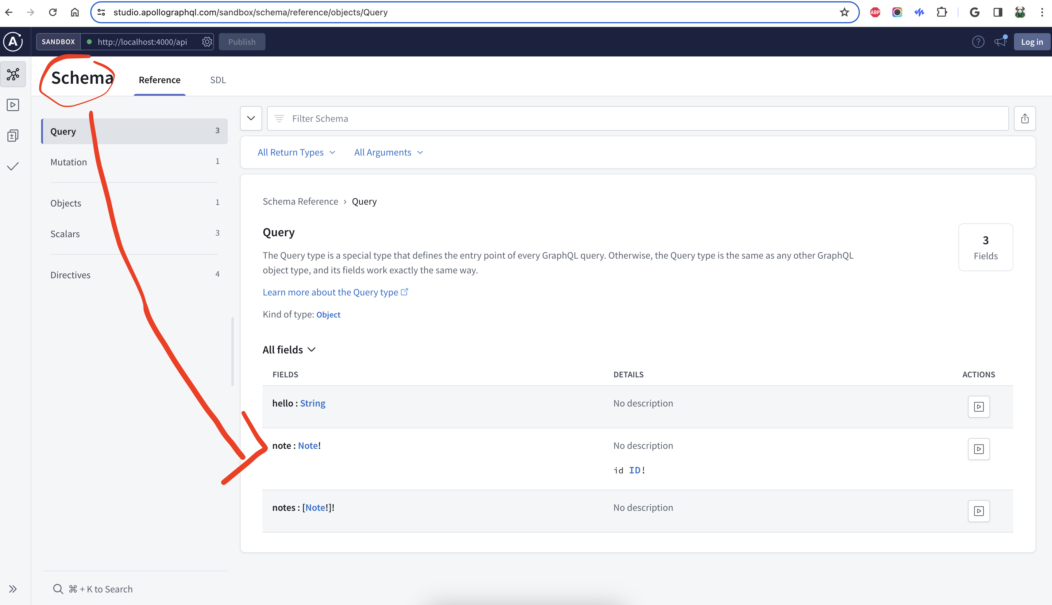
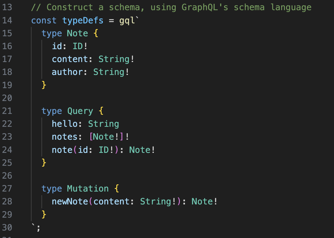
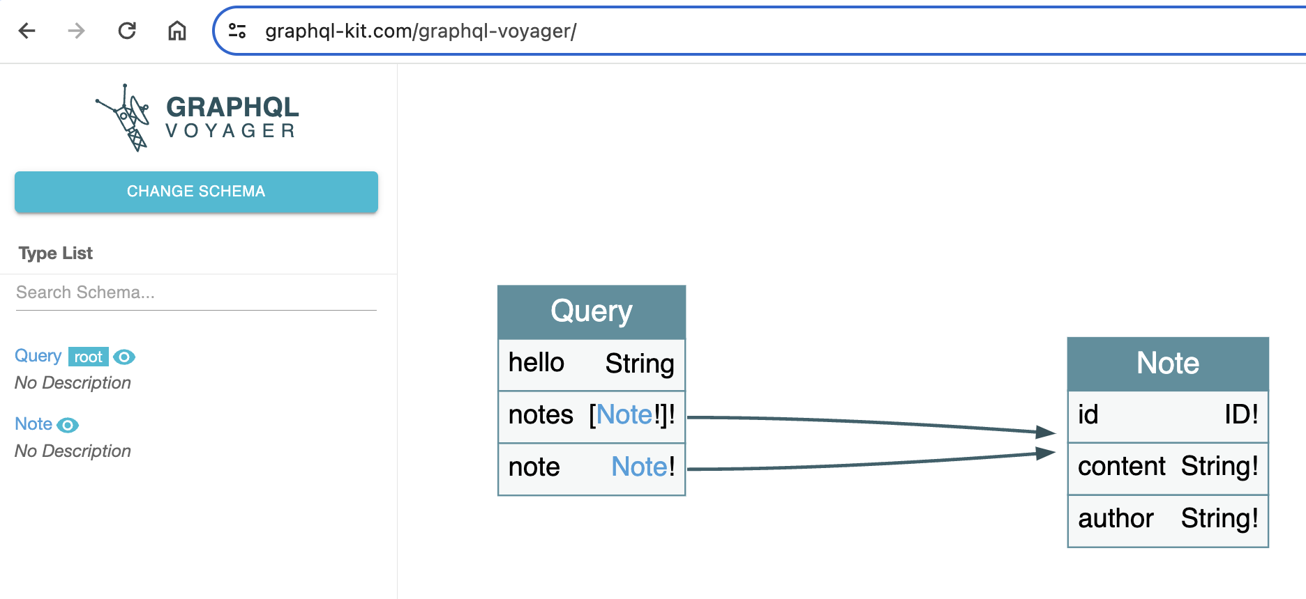
Just like a SQL table, one needs to know the schema of the data first before using it. Above is a screenshot of the GraphQL schema visualized in apollo explorer.

We know there are 3 fields (columns) that we can query, the hello field will return helloworld for testing purpose, notes to return a list of all the notes and note to return a specific note.

In this simple example, there are 3 fields available to query, and each field can have 3 attributes that you can customize. Depending on the use cases, some users may only need the content, some may only need authors, some may need all fields, if you take all the combinations of different user cases into account, it is very hard to expect all the users cases. Instead, GraphQL defines the schema with all the ingredients available, and the users just need to query what they need.

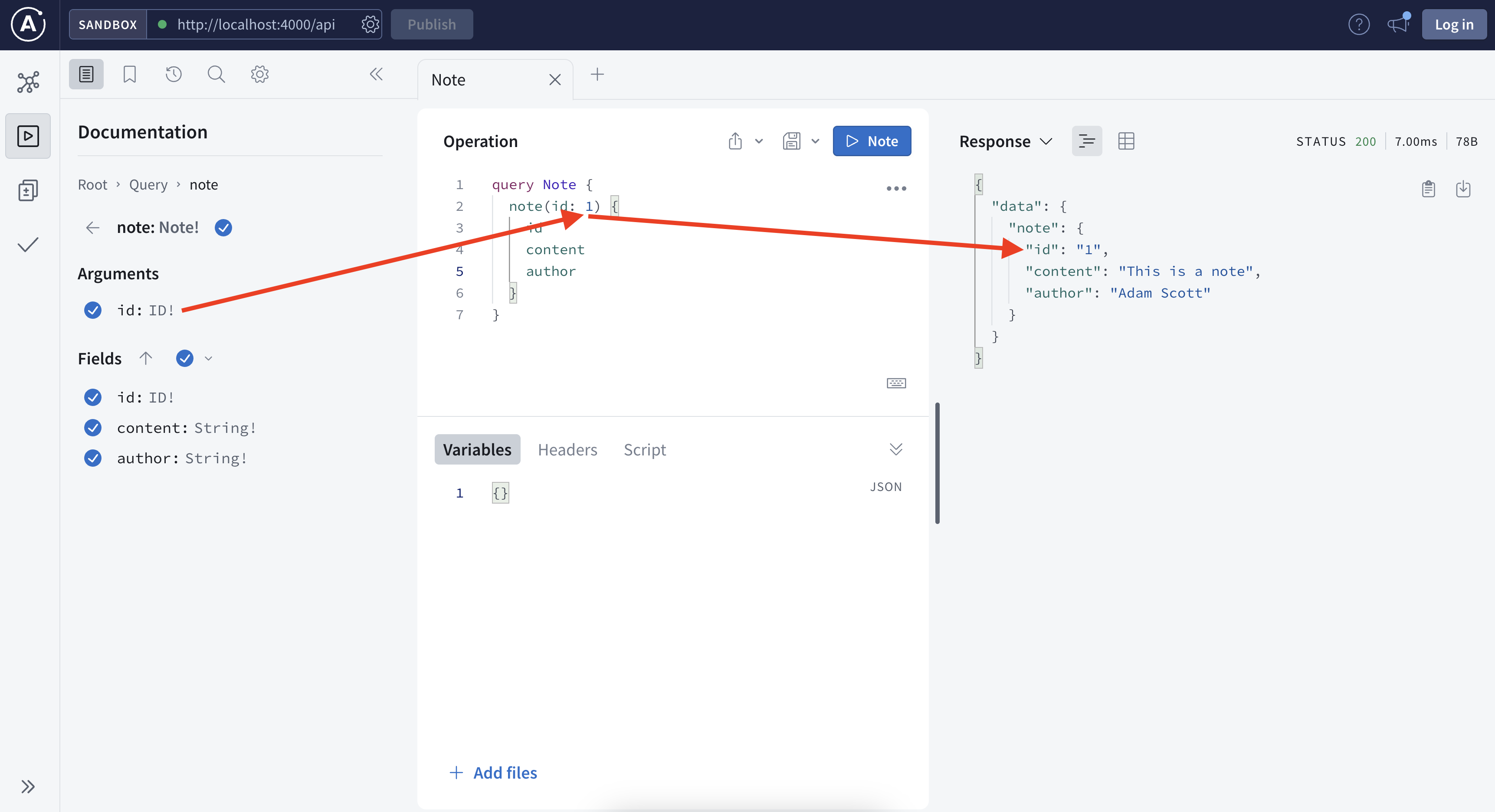
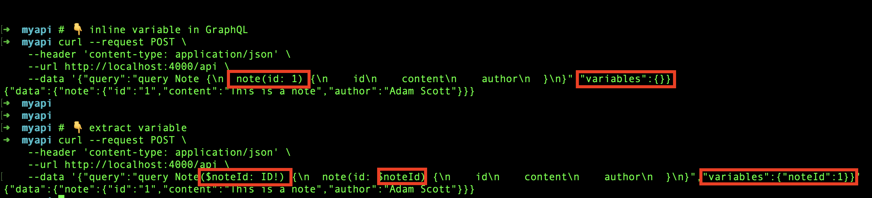
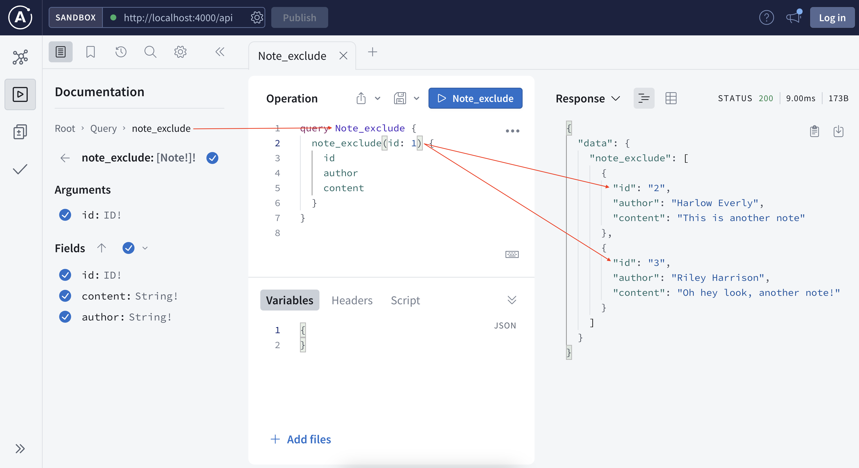
The explorer is very helpful to interact, by nature, it is just a typical HTTP request with the graph query in a json format stored in the payload. See below, you can also choose between inline variable or extract variable and both works.

How to Build it

Define Schema

gql“ in Javascript represents a tagged template literals, it parses the GraphQL schema language the typeDefs object will need to be passed to the apollo server during initialization.

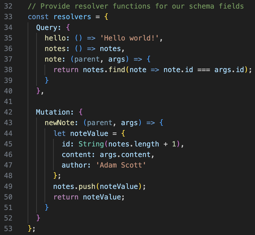
Define Resolver

The schema defines the “what”, and the resolver takes care of the “how”. In this simple example, the Query block defines how the three query works.

Try it Yourself

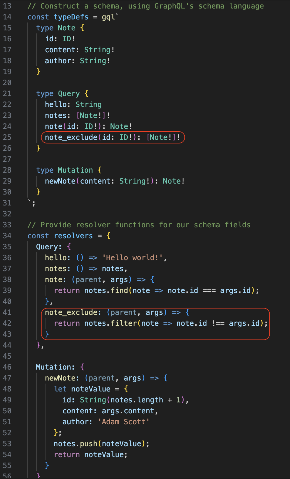
Now we saw how the schema and resolver work together. Let’s try to add a new field so it returns all the notes but the one specified by the user (this may apply to feed new unread articles).

Where is the Graph

We just covered the query language part, now let’s think about where is the graph. There is a great article by Bogdan discussing about the graph part of GraphQL.

You can also visualize any graphql using a tool called graphvoyager.

More Questions

• if graphql query ended up being a DAG, given different steps might take different time, is this also an optimization problem as there may be a goal of minimizing the total execution time or maximizing the total throughput, aka, the job scheduling problem.

Luna Dong Podcast – Building the Knowledge Graph at Amazon with Luna Dong
Three key features of Knowledge Graph:
1. structured data (entities and relationships)
2. canonicalization/rich/clean
3. data are connected
In Amazon, there exists separation of digital product from retail products because the former tend to have better and more well structured metadata, the retail products tend to require to extract digital data from various kinds of real life data for example (images, raw texts, …)

“is-a” relationship, “event” information, use the “seed knowledge” to automate the building of train data. The more you know, the faster you learn.

Knowledge Extraction: from web, product description (text, …) web tables, product data is collected from text and images

Data Integration: “is_a_director_of” is the same as “director” relationship, database and NLP community, we put things together to decide whether two things are wrong by looking into inconsistency (color, product flavor, data sources). Data fusion is to decide which version is right – is this person’s birthday on Feb 28th or Mar 28th? Through this process, you can learn embeddings that can be used for downstream tasks like search, recommendation, Q&A and many others.

Human in the loop is important because we need high quality data, it is important to seed the training data, annotate the data and calibrate and analyze the overall performance, and it is also important to address the last mile failure if we want to be 99% accurate.

The most inspiring moment from Luna is from Amazon’s fulfillment center, to combine machine power and human power.

Data acquisition: the product manufacturer’s website contains a lot of information, start with general crawling and sometimes do targeted crawling. It is not a binary, it is a mixture.

Embedding: conditional embedding. spicy is a valid flavor, spicy is unlikely to be part of an ice cream flavor, capture these constraints in an implicit way, these spicy flavor in general can be covered in certain types of products.

Triple – subject-predicate-object, look at all the triples together, and clean the embeddings from that way, the embeddings can propagate in the graph. Some products have the flavor spicy. Graph neural network is one of the most effective way to solve the problem.

The knowledge graph is a production system, the knowledge is generated from a lot of products – there are three major applications – search (intent), recommendation (similarities but still some difference), display of information (structured information and structured knowledge, better comparison table).

Luna said most knowledge graphs are built and owned by large corporations, she wishes there are tools for smaller business. She said there are three levels, first being the database and tooling storing knowledge graphs, the second being the techniques to entity and relationship extraction.

Open knowledge is an effort to connect and hook up different data sources.

I am trying to figure out a way to do real time transcribing and managed to got open ai whisper run and running. This post is for me to write down what I did and some of the learnings.

Download Content

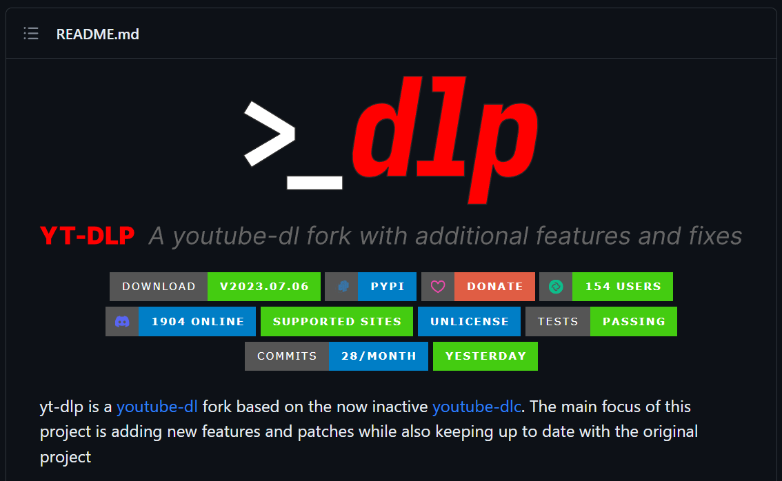
The first thing you need is content, the quickest way is of course to download the content from youtube. There are many online tools that can help save you some key strokes. However, if often you need to work with youtube videos, it saves you more time by figuring out a programmatic way. I found two libraries that worked well for me, the youtube-dl and yt_dlp.

It is very convenient to use it.

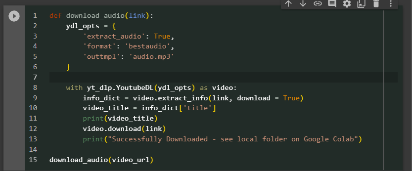
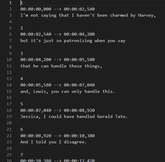
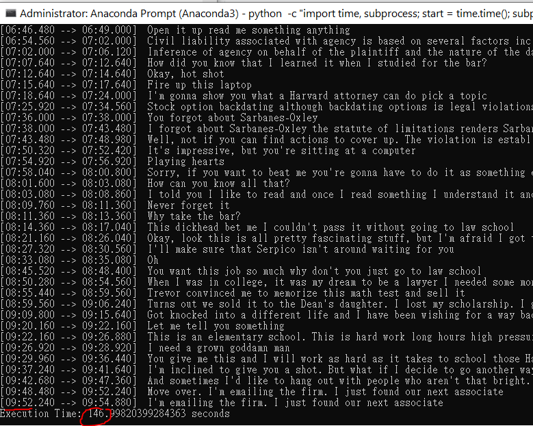
now you got 10 minutes good quality of a youtube audio and yt_dlp also supports download video with various options. (below is a screenshot of a 10 minutes video, the 1st scene of the TV show suits). This TV shows is spoken in American English quite fast paced and contains unfamiliar terms often because its plot is about stories between lawyers.

Install and Set up Whisper

This step takes me a bit longer than expected.

download the right whisper

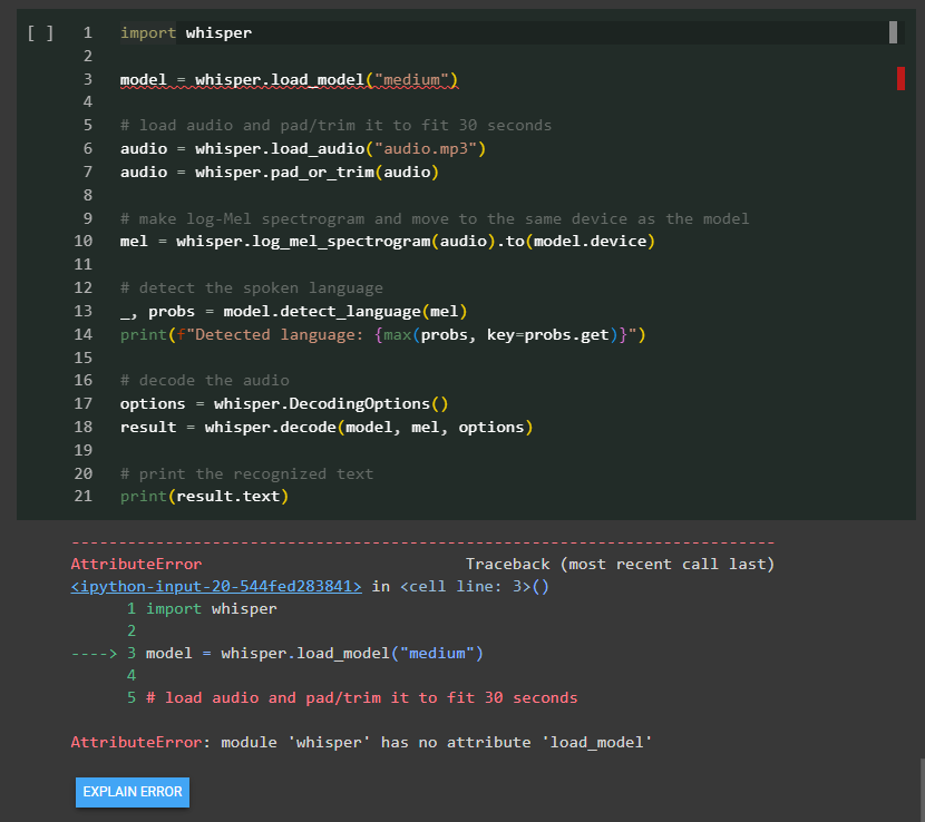
I tried to run the tutorial from whisper documentation but couldn’t seem to get the first step running – call the load_model method. It turned out there is a discrepancy between the whisper library in pypi and the latest in github, the best way is to point pip to the github official account and you should be good to go. eg. pip install git+https://github.com/openai/whisper.git. Otherwise, you should the same error message as me below.

set up torch gpu correctly

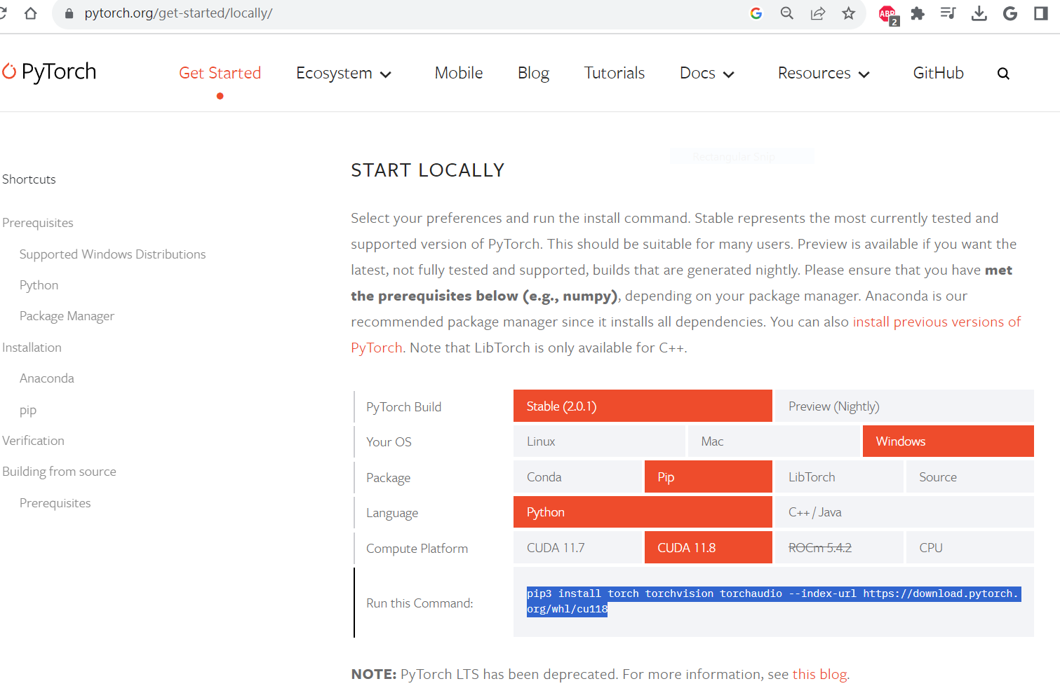
whisper uses pytorch behind the scene, whisper offers you the option to run either cpu or gpu. In order to do it, we have to make sure the pytorch is properly installed and set up with the gpu enabled. Long story short, you should really follow the documentation from pytorch’s website. Otherwise, you can easily run into problems of installing cpu only version, outdated version, with the wrong cuda version or simply the wrong package (pip install torch, NOT pytorch)

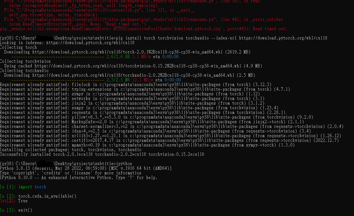
For me, I had to uninstall torch all together first, then follow the pytorch site’s instruction to reinstall again. The installation is a bit time consuming downloading the 2.6GB from wheel for windows. For the first time, it even failed half way through but the second time is the magic. In hindsight, one could relax the timeout to avoid slow downloading related error. After all, you can run the code below to confirm the GPU is working perfectly with pytorch.

get the model

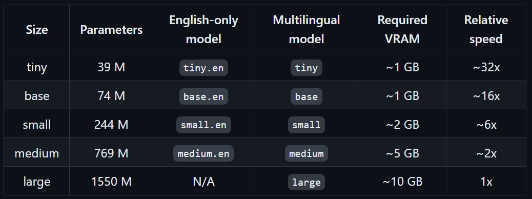
Whisper has a few different models, the bigger model has better performance but comes at the cost of a bigger size (storage/ram/network) and slower speed. Just keep in mind that the model will be downloaded the first time it is being used and you should expect a delay depending on your network.

transcribe

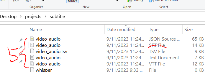
transcribe is as easy as “whisper audio.mp3”, in the end, you get 5 files.

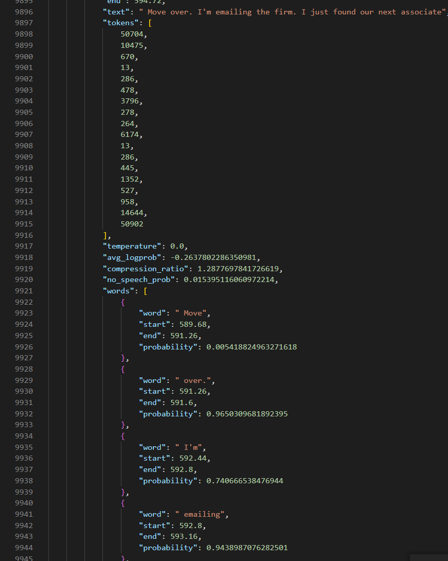
By enabling the word level timestamp “–word_timestamps True”, you can even get the word level prediction.

computing performance

To measure the performance, I have to write up a small python script given windows lacks a timer like the time in Linux.

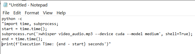
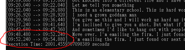
By using a GPU, it took 146seconds to transcribe 9:54 contents, which the ratio is about 3.9x. The bigger this ratio, the faster it is. By using cpu, it took 2001 seconds which is only 0.29x. Using GPU leads to a 10 times performance difference.

description	time (s)	speed (time/594s) (“how long it takes to transcribe 1s”)	throughput (594s/time) (“in 1s, how long it can transcribe”)
medium gpu	146	0.25	4x
medium cpu	2001	3.37	0.3x
tiny gpu	48/50	0.08	12x
base gpu	40/40	0.07	15x
large gpu	783/800	1.31	0.75

Summary

The overall experience working with whisper is quite pleasant, the setup, performance (computing and transcription quality wise) are definitely outstanding. This makes it a useful tool for many applications and if designed properly, the base model can be used for real time transcription.

Agent is a key component in langchain that serves the role of interacting with llm and execute tasks leveraging tools. This article documents my experience following this tutorial.

There are many types of agents in langchain, eg. conversational, functional, zero-shot react etc. In this example, we will be using openai functional. At a high level, openai function is an extension to the basic GPT LLM, it feeds a self-defined function to openai, openai will understand what it does and when to use it, through a natural language way, openai will parse the given questions, decide to answer the question requires invoking the user defined function, if so, it will return the parsed arguments and execute by calling the function. This is a good offering because there has been many scenarios where it is best to use specific tool to ensure the determinism by avoid hallucination that comes with language model.

Tutorial

Instead of using the simple count letter example included in the tutorial, the first change I made is to test out what if there are two arguments in the function, interested in seeing whetheropenai function will be able to successfully extract and assign accordingly.

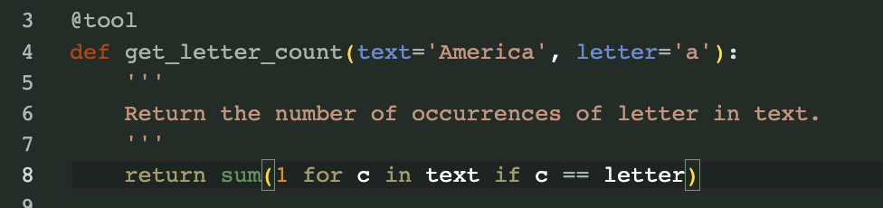
The tool decorator will register your function so that openai can recognize it. The doc string is also a required field to guide openai what is it used for and when to invoke it.

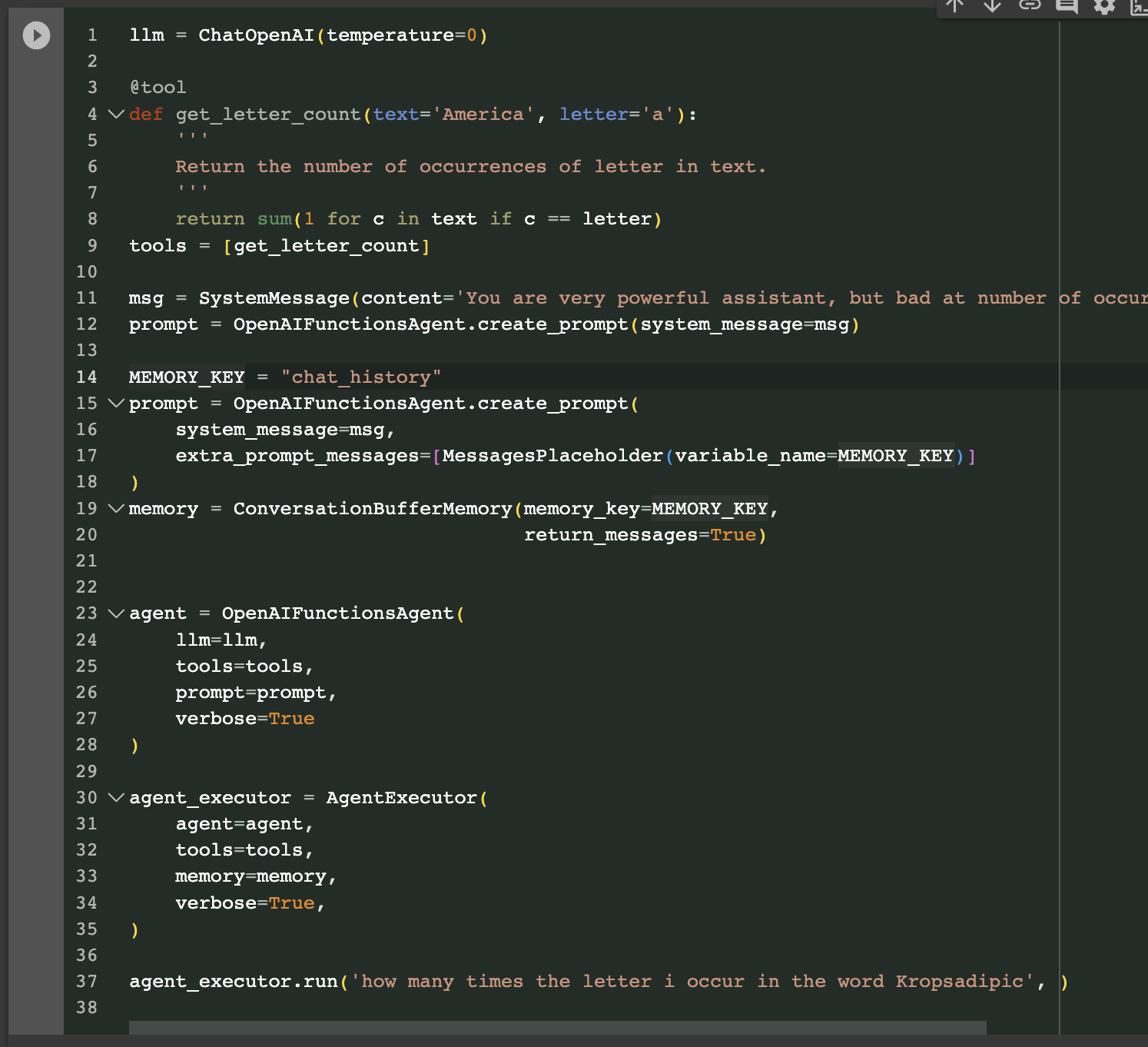
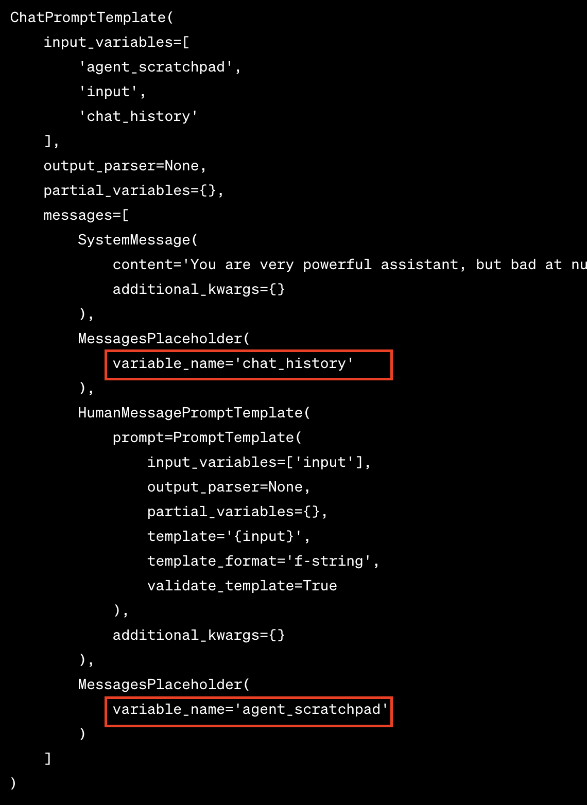
The agent creation requires the LLM, tools and a specific OpenAIFunctionsAgent prompt.

You can turn on the debug model by setting langchain.debug = True. When the debug mode is enabled, you see a lot of messages are being captured and returned to the screen.

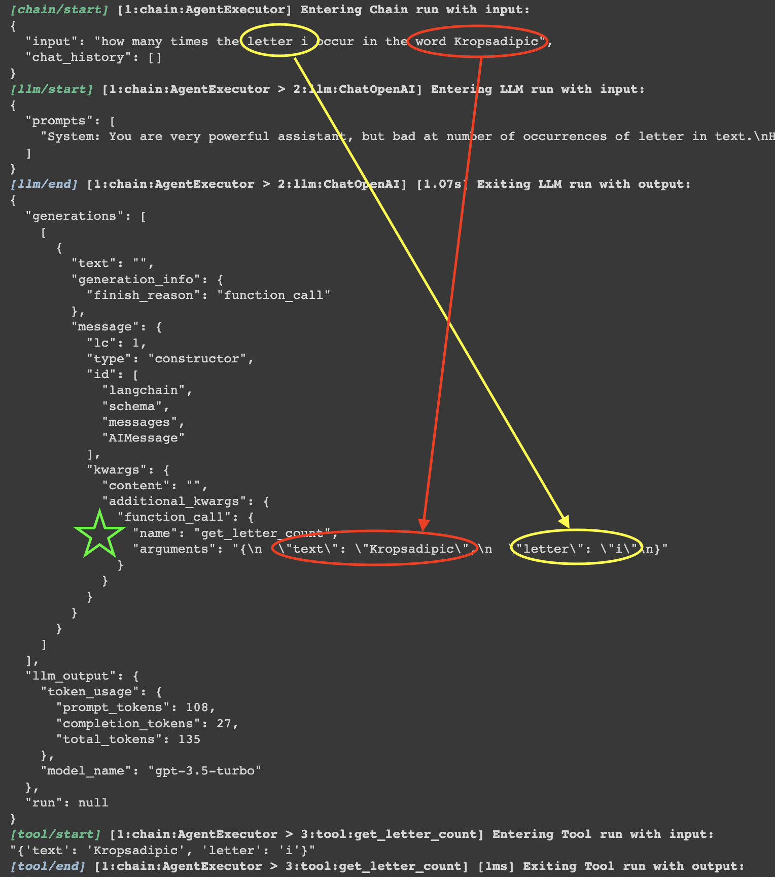
Based on the debug messages, the question is being successfully parsed, and openai understands my question, realize its limitations of counting letters, decided to call the get_letter_count function and successfully parsed the question to extract the right both arguments (see screenshot above).

Code Dependencies (DAG of variables/functions)

There are indeed several steps in this simple example but most of the code are just boilerplate that you can simply copy and paste in your application, to visualize the inter-dependencies within all the components, here is a visualization in graphviz dot:

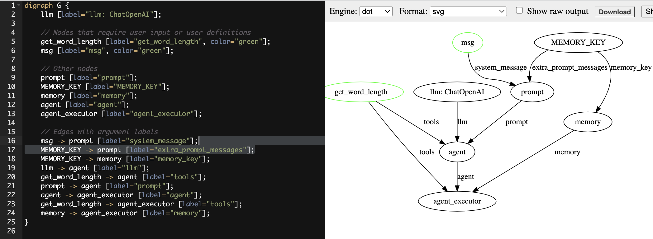
Based on this visualization, the only two places that requires your customization is the original function that you need to teach openai, and a basic system message that you guide openai under which scenario should the function be invoked.

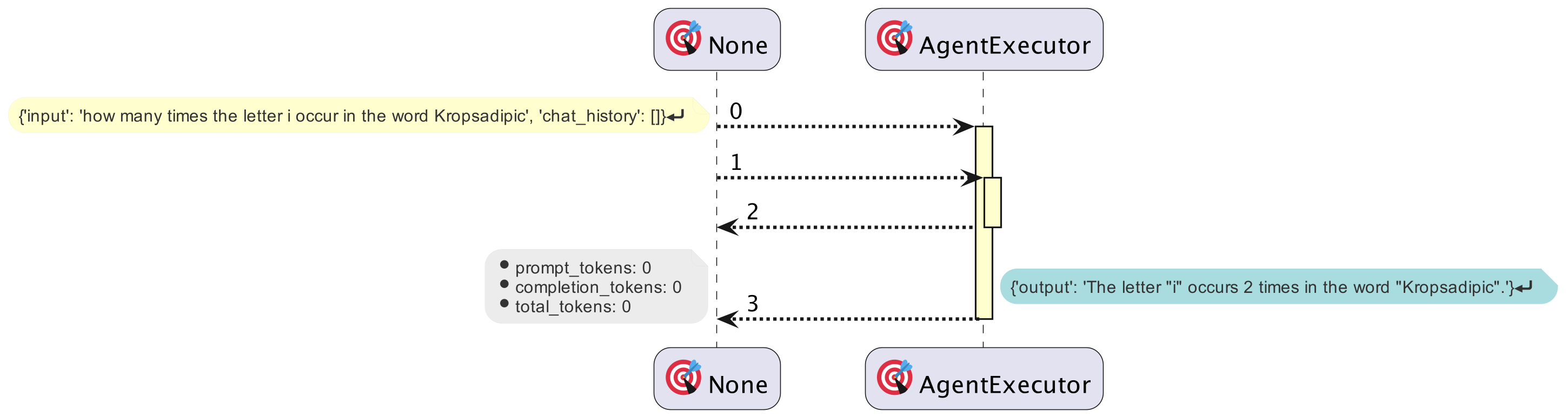
Visualizing using PlantUML

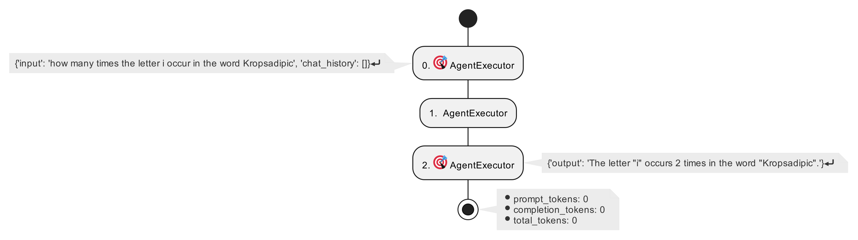
If you are interested in the execution sequence and activity, there is a library called langchain-plantuml that will using the callback method to capture all the events and later visualize it in this beautiful graphy way. On a side note, plantuml is a

Activity

Sequence

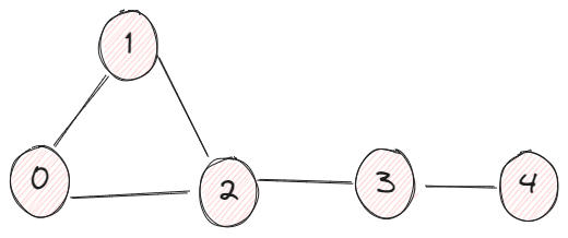
So, let’s use a simple example to demonstrate:

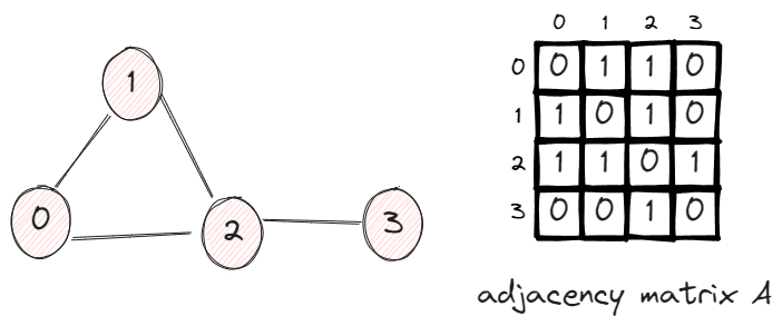
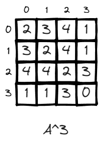
In this graph, we have 4 vertices and 4 edges. The adjacency matrix A has the value Aij = 1 if two vertices are connected, otherwise 0.

Walks of length n

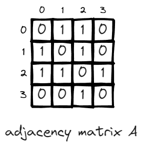
n = 1 is the first scenario, there is one walk between two nodes if they are connected, this is essentially the definition of adjacency matrix.

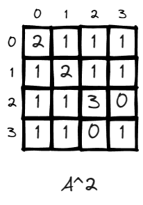
n = 2, the value of matrix changed, some values go up like (v2,v2) changed from 0 to 3. This is very intuitive. It means there doesn’t exist a path to walk from v2 back to v2 in one step, and there exit 3 paths if given two steps. (2>1>2, 2>2>2, 2>3>2).

n = 3, (v2, v2) now becomes 2, it means there exist 2 paths to leave v2 and return to v2 in 3 steps, which is 2>1>3>2, 2>3>1>2.

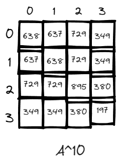
n = 10, just for fun, there exists many more paths when the power is high. V3 has the lowest number of paths likely due to it is a dead end within only one edges connecting it to the rest of the world via v2. And v2 has the highest number of returning to it self because it has the highest degree and is the central node of the graph.

In fact, the matrix multiplication is an exhausted approach to iterate through all the possible permutations of paths, for a unweighted graph, if a path exists, the value of all the edges of that path will be 1 and multiplication of these paths will be 1.

The matrix multiplication approach is basically a breath first tree search

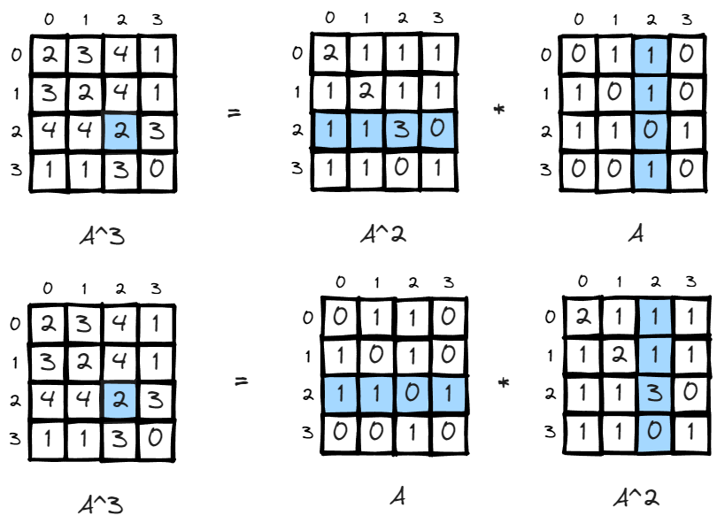
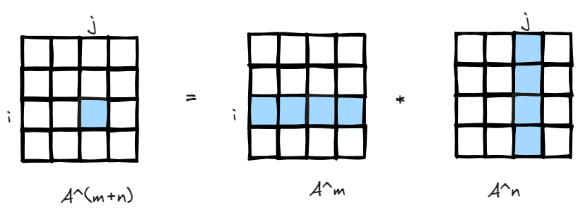
Since matrix multiplication is association, (A*B)*C=A*(B*C), the interpretation is also easy to understand, if there is a matrix storing how many paths there are leaving i to all other nodes in m steps, and another matrix storing all paths returning to j from all other nodes in n steps, you got the total number of paths leaving i return to j in m+n steps.

n being distance if it is first time An(i,j)>0

This is less straightforward, and the previous example of 4 vertices is not a good example to demonstrate this property because everything is so close to each other, so I added another node v4.

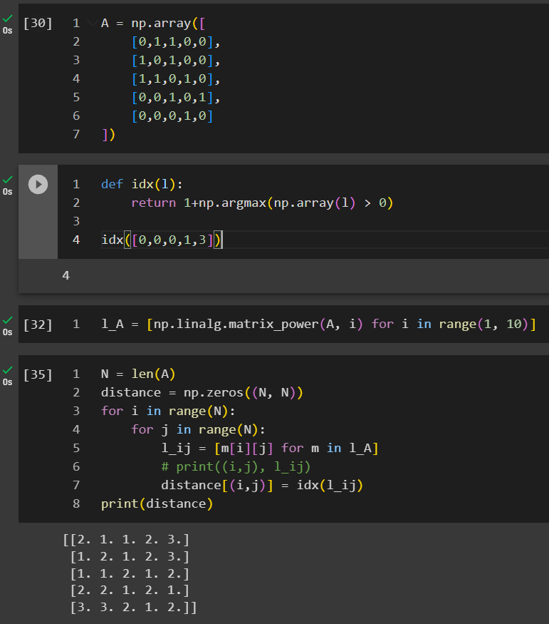
In this example, we created a list of l_A where it stored all the matrices when n increases from 1 to 9. We are looping through all the cells to identify under which n that An_ij first time becomes positive.

In conclusion, adjacency matrix has such interesting properties and it is symbolically simple, however, it is full permutation under the hood and likely won’t scale well to large graphs, so better algorithms or optimization is required given your application.

A key step in preprocessing prior to training a model is to properly split the dataset into training, validation and test datasets. In traditional machine learning, the dataset is usually a dataframe/table like where each column represents a feature and each row represent a record. Due to the simplicity in that structure, the split can be as easy as rolling a dice to determine which records goes to which bucket, you can find the source code for sklearn model_selection.train_test_split. However, the data structure for a graph dataset is different, it contains nodes and edges, in addition, it contains attributes and labels for nodes and edges. For a heterogenous graph, it can be more complex with different types of nodes and edges. Given those challenges, torch_geometric is “battery-included” with a function train_test_split_edges for edge prediction. In the latest documentation, train_test_split_edges is deprecated and is replaced by  torch_geometric.transforms.RandomLinkSplit, in this post, we will only cover train_test_split_edges due to its simple implementation. Before we dive into the specifics, let’s first take a look at popular ways of splitting data and its best practices.

Cora

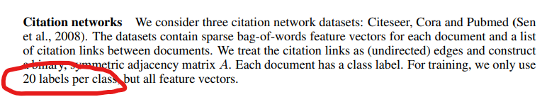
Cora dataset is a popular graph dataset. it describes the citation relationship between scientific publications, there exists 5429 links and 2708 entities and 7 classes representing a domain the publication belong to.

GCN (graph convolutional network) has been considered a bedrock for graph machine learning, in the paper where GCN is being considered invented – semi-supervised classification with graph convolutions networks. The author Kipf and Welling used the cora dataset.

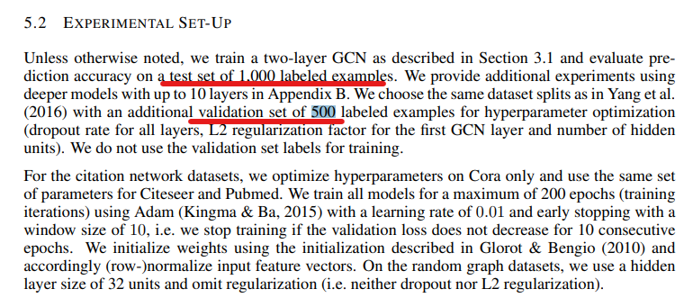
However, instead of using all the links for training, they only picked 20 samples per class, given there are only 7 domains, the training dataset is only 140 records which is merely 2% of the whole dataset. And they used 500 (9%) for validation and 1000 (18%) for testing. The volume of training data can even be considered disproportional comparing to most supervised learning where very majority of the data goes to training if not all.

This is a common practice in semi-supervised learning on graphs, where the goal is often to learn from a small amount of labeled data (the training nodes) and to generalize this to the unlabeled data (the test and unused nodes).

This may not be a perfect example as it is a node classification problem but it is a good conceptual example demonstrating it is critical to preprocess the dataset by splitting them right.

Next, let’s take a look at for a link prediction task, how to split the links into train, validation and test.

train_test_split_edges

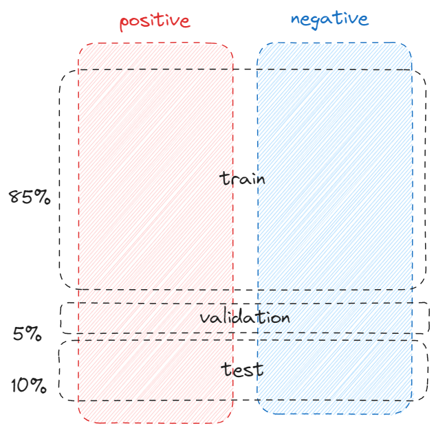
By default, train_test_split_edges splits the dataset into 3 categories, 5% goes validation, 10% goes to test and the rest 85%=1-5%-10% goes to training. However, the link prediction is a binary classification by nature, so we need to have positive cases (relationship exists between two nodes) and negative cases (relationship doesn’t exist between two nodes).

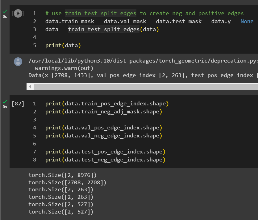
If the dataset is already loaded into torch_geometric, you can just run train_test_split_edges on the data object.

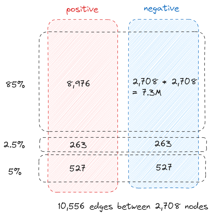
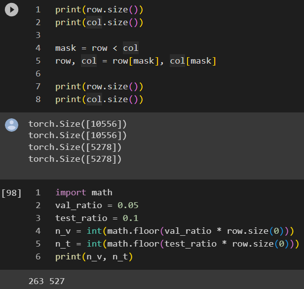
An interesting observation is that the validation and test edges is 2.5% and 5% of the total edges instead of the 5% and 10% we previously mentioned, soon you will know why.

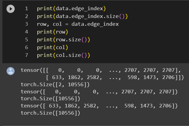
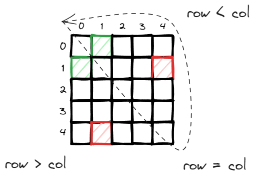
row stores all the source node of all the links and col stores all the destination nodes. They have the same size as the number of links which is 10,556. Consider there are 2,708 nodes, technically the adjacency matrix should have the size of 7.3M, 10,556 is only 0.14% of 7.3 million so storing the links in this way (COO – coordinate format) is very efficient.

in an undirected graph, you can consider either direction and it is efficient to consider only half of the adjacency matrix, in this case, the top right upper triangle (diagonal is self directed link which can be ignored).

Below is the implementation, the concept is very straightforward and in addition to the index for train/validation/test, if the edge attribute is available, it is also stored in the corresponding edge_attribute.

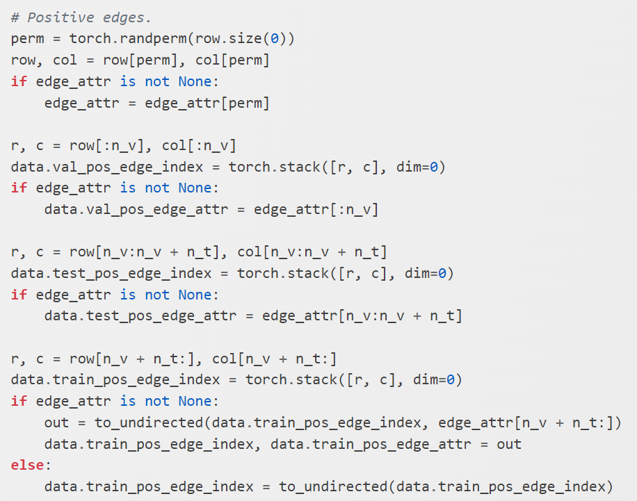
The negative samples are handled differently due to the fact that what is not there implicitly considered negative samples, and it is usually 100x bigger if not 1000x than the positives samples.

First, they construct a full adjacency matrix where each cell has the value of one. And then mark all the existing edges as 0 and find all the remaining ones as negative samples. Then it extracts all the indices using tensor.nonzero.

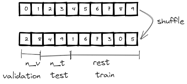
From the negative samples, it first extracts n_v + n_t many samples as negative samples which corresponds to the same number of samples for positive validation set and test set. After that, it update the neg_adj_mask to exclude those allocated samples.

This is the beauty of this technique. There are significant amount of negative training samples. Instead of storing them like positive samples or negative validation set and test set, we decide to keep track of the huge population by using the neg_adj_mask instead of COO format, this way.

negative sampling is an important step to identify negative training datasets that can be used for training and generate embeddings. In fact, it is such an important engineering practices that otherwise, it will be extremely computational difficult to calculate embeddings in simple techniques like randomwalk and others.

In the lecture 3.2-random walk approaches for node embeddings by Prof. Leskovec, he explained really well how random walk requires a normalization step that in theory requires V^2 computational complexity but can be approximated using negative sampling to k * V (in practice, k can ranges from 5 ~ 20).

The concept of negative sampling is not limited to graph, it is used in NLP – word2vec explained.

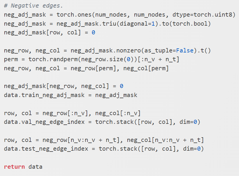
In order to do negative sampling in pyg, you can just call the negative_sampling function under torch_goemtric.utils. The only input it required is the edge_index which is a tensor containing the pairwise edges between from and to nodes.

In this example, the graph can be represented by the adjacency matrix. It is sparse and usually sparse because there exist only 4 edges out of 16 (V^2) possible edges. The rest of the nodes are implicitly negatives edges, edges that don’t and shouldn’t exist. The negative_sampling as default will return the same number of negative edges as the number of positives edges. In this case, it returns the four zeros (highlighted in green).

Also, if you pass a tuple (n,m) to the num_nodes, it indicates a graph is a bipartite graph where the number of sources nodes is n and the number of destination nodes is m. The adjacency matrix will be adjusted to n*m instead of n^2. The negatively sampling logic remain the same, it still returns 4 negatives edges that should not exist.

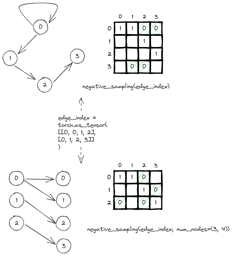
There is also a batch negative_sampling, the only difference is that you can pass in a batch parameter in order to distinguish which graph certain edges belong to. The negative sampling will only occur within the same graph instead of cross graphs.

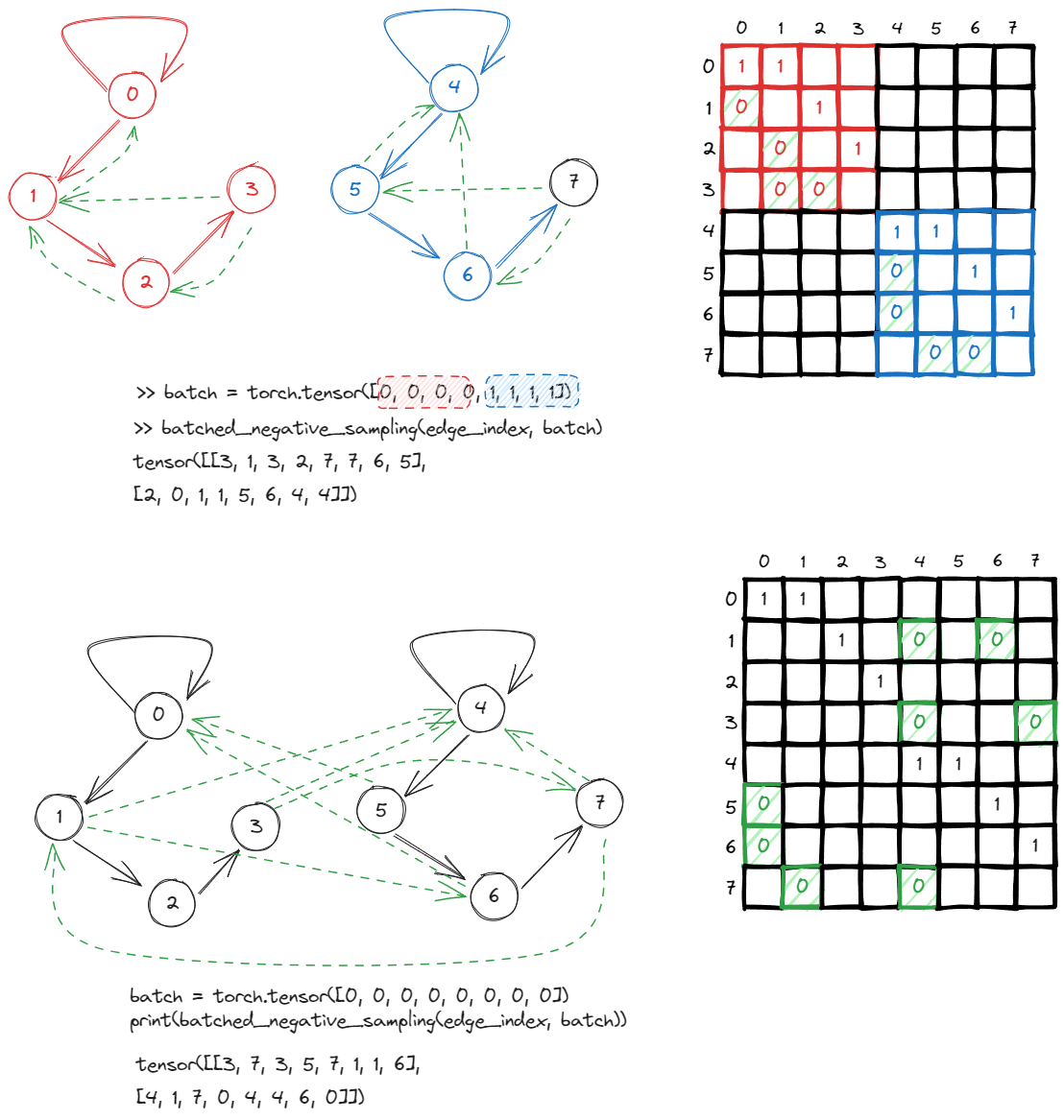
To demonstrate, to treat the two graphs as one graph, you can simply ignore the the batch parameter and immediately, one start observing negative samples crossing graphs.

I found the chatgpt’s explanation easier to understand.

“

In your example, the batch tensor is torch.tensor([0, 0, 0, 0, 1, 1, 1, 1]). It means you have a batch of two graphs. The first four nodes (indices 0, 1, 2, 3) belong to the first graph (batch 0), and the second four nodes (indices 4, 5, 6, 7) belong to the second graph (batch 1).

So, when you’re using batched_negative_sampling(edge_index, batch), this function will generate negative edges (non-existing edges used for training graph learning models) while making sure the nodes of these negative edges are within the same graph. In other words, it will not generate a negative edge between nodes from different graphs.

“

analysts have always been a highly demanded job. Business users and stakeholders needs facts / insights to guide their day to day decision making or future planning. Usually it requires some technical capability to manipulate the data. This can be a time consuming and sometimes frustrating experience for most people, everything is urgent, everything is wrong, some can be helpful, and you are lucky if this exercise actually made a positive impact after all.

In the old world, you have your top guy/gal who is a factotum and knows a variety of toolkits like Excel, SQL, python, some BI experiences and maybe above and beyond, have some big data background. To be a good analyst, this person better be business friendly, have a beta personality with a quiet and curious mindset, can work hand in hand with your stakeholders and sift through all the random thoughts and turn it into a query that can fit into the data schema.

In past few years, there has been improvement in the computing framework that many data related work is democratized to a level anyone with a year or two engineering background can work with almost infinite amount of data at easy (cloud computing, spark, snowflake, even just pandas, etc), there are tools like PowerBI, Tableau or Excel that can have people query well formatted data themselves and even innovations like Thoughtspot, Alteryx, DataRobot to make it a turn-key solution.

Recently I came across a demo using langchain. Without any training, the solution can generate interesting thoughts and turn natural languages into working queries with mediocre outcomes.

Set Up

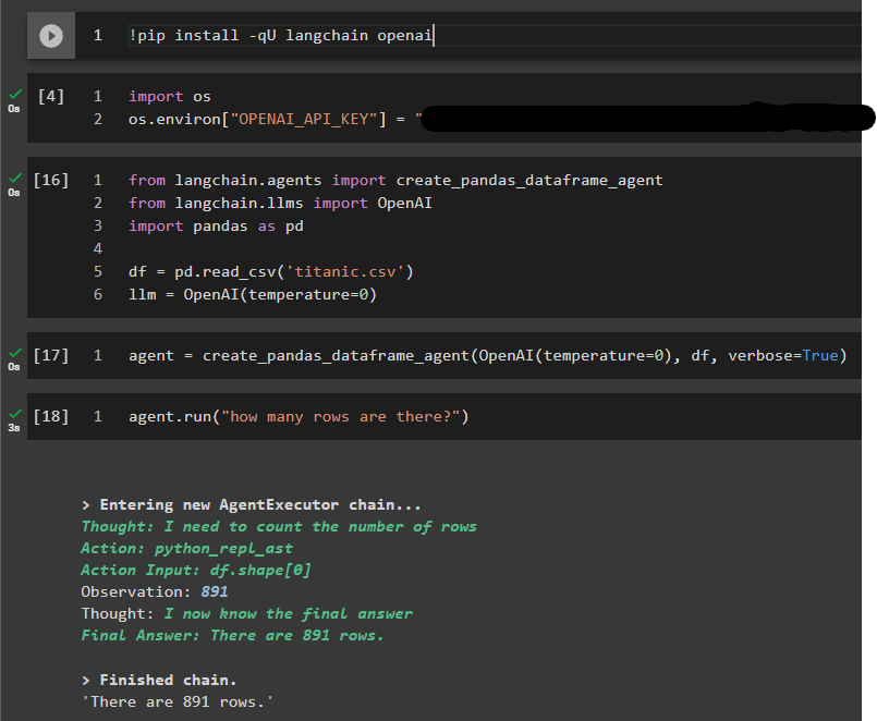
The setup is extremely easy, sign up to an OpenAI account, download langchain and that is it.

Once you create an agent, you can just call agent.run and ask any question you may have in plain language.

To confirm everything is working properly, we asked “how many rows are there” and got the answer of “891” for the titanic dataset.

Interesting Questions to Ask:

Schema

To get started, you can ask about the schema, typically people will do df.describe(), df.info() or df.dtypes

As the number of columns increases, it is sometimes time consuming to navigate and find the date column types, you can now just ask the dataset yourself.

Filter

Thanks to openai, they even support multilingual. If you ask the question in Chinese, it will reply back in Chinese.

Aggregation

Correlation

Visualization

Machine Learning?

Not Perfect

There is an interesting observation that I asked the question of “how many women survived”, and I came across 3 different answers for the exact cell that I executed before. The first time I executed, the answer is wrong as it only returned how many females were aboard without taking into the survivorship, then after several other questions, the same answer got asked and somehow it returned 0. When I restarted the prompt by recreating the LLM, I got the correct answer.

Again like any other solutions, “Trust but verify”